Module 4: Logistic Regression
Module Overview
In this module, you will transition from regression to classification with logistic regression. You'll implement train-validate-test splits, understand classification baselines, and learn about scikit-learn pipelines. These skills will enable you to build and evaluate models for binary classification problems.
Learning Objectives
- Implement a train-validate-test split
- Begin with baselines for classification
- Express and explain the intuition and interpretation of logistic regression
- Use scikit-learn to fit and interpret logistic regression models
- Use scikit-learn pipelines
Objective 01 - Implement a train-validate-test split
Overview
In the previous module we used a train-test split, where we hold back a subset of the data to use for testing the model. When we train a model we also need to evaluate the model. Recall that if we evaluate on the training data we're not getting an accurate estimate of the true performance of the model. For this reason, we need to use test data that the model has not yet seen.
Sometimes it's useful to be able to have an intermediate step where the model can be evaluated without using the set-aside test set. This is where a validation set is useful. Consider the situation where we take a subset of our data and set it aside as the test set - we won't touch this data until we're ready to evaluate a final model.
With the remaining data, we can divide it into training and validation sets. We then train the model on the training data and evaluate it on the validation data. Another advantage of using a validation set is that it can be used to tune the model or adjust the hyperparameters. Iterations of tuning and model fitting are used to find the final model, which is then evaluated using the test set.
Train-validate-test
Some general definitions are:
- training dataset: the sample of data used to fit the model
- validation dataset: the sample of data used to evaluate the model and possibly to adjust the hyperparameters
- testing dataset: the sample of data used for final model testing; not to be used for anything other than testing so that the result is unbiased
One last point to make is that sometimes you won't even have access the test set! If you are participating in a Kaggle competition, for example, you cannot view the actual target values for the test data, and can only generate the predictions for your submission. The number of test prediction submissions might be limited, or you might not want to make numerous test submissions just to evaluate or tune your model.
In this next section, we'll create our own train-validation-test data sets. We'll follow the guideline of using 60% for training, 20% for validation, and 20% for testing.
Follow Along
We haven't yet worked with the Iris dataset in this module, so we'll
start there. In the following example, we load the data and then
separate out the feature petal_width and the target
petal_length. Having plotted this data earlier, we know
there is a linear relationship between the petal width and length: the
wider the petal, the greater the length. We'll use a linear model to
predict our target.
# Import numpy and seaborn
import numpy as np
import seaborn as sns

iris = sns.load_dataset("iris")
display(iris.head())

x = iris['petal_width']
X = np.array(x)[:, np.newaxis]
y = iris['petal_length']
| sepal_length | sepal_width | petal_length | petal_width | species | |
|---|---|---|---|---|---|
| 0 | 5.1 | 3.5 | 1.4 | 0.2 | setosa |
| 1 | 4.9 | 3.0 | 1.4 | 0.2 | setosa |
| 2 | 4.7 | 3.2 | 1.3 | 0.2 | setosa |
| 3 | 4.6 | 3.1 | 1.5 | 0.2 | setosa |
| 4 | 5.0 | 3.6 | 1.4 | 0.2 | setosa |
First, we'll hold back a subset of the data just for the test data. We'll do this with the scikit-learn utility. We'll call it something different from "train" so that we don't confuse it with the actual training data later.
# Import the train_test_split utility
from sklearn.model_selection import train_test_split

# Create the "remaining" and test datasets
X_remain, X_test, y_remain, y_test = train_test_split(
    X, y, test_size=0.2, random_state=42)
Then we'll create a training set and validation set from the remaining data. We could have done this in one step but we're breaking it down here so it's easier to see that we removed a test subset and will not accidentally use it for evaluation until we're ready to test.
# Create the train and validation datasets

X_train, X_val, y_train, y_val = train_test_split(
    X_remain, y_remain, test_size=0.25, random_state=42)

# Print out sizes of train, validate, test datasets

print('Training data set samples:', len(X_train))
print('Validation data set samples:', len(X_val))
print('Test data set samples:', len(X_test))
Training data set samples: 90
Validation data set samples: 30
Test data set samples: 30
Now we can fit our model and evaluate it on our validation set.
# Import the predictor and instantiate the class
from sklearn.linear_model import LinearRegression

# Instantiate the model
model = LinearRegression()

# Fit the model
model.fit(X_train, y_train)

# Use the VALIDATION set for prediction
y_predict = model.predict(X_val)

# Calculate the accuracy score
from sklearn.metrics import r2_score
r2_score(y_val, y_predict)
0.9589442606386026
Well, that's a pretty good model score (R-squared), which we expect because we know the Iris dataset has a strong linear trend between the petal width and petal length. Now would be the time to change any of the model hyperparameters and evaluate on the validation set again. We'll continue with the default model parameters for now. Hyperparameter tuning is something that will be introduced in the later Sprints.
Now, let's use the test set we held back above.
# Use the TEST set for prediction
y_predict_test = model.predict(X_test)

# Calculate the accuracy score

r2_score(y_test, y_predict_test)
0.9287783612248339
The R-squared score is a little lower than it was for the validate set. If we were to run the model and test again with a different random seed, the scores would be different and the test score might be higher.
Challenge
Using the same data set as in the example, try changing the
random_state parameter to see how the validate and test
model scores change.
Additional Resources
Objective 02 - Begin with baselines for classification
Overview
When we fit a model to our data and look at the model score, we need something to compare that score with. As we covered in module 1, a baseline is a simple estimate or prediction for a model. A baseline can be determined from descriptive statistics such as the mean value of a variable, or even a simple linear regression for two variables. We started by finding a baseline for a linear regression problem where we were predicting continuous variables. From our penguin data set we used a baseline estimate of the ratio of flipper length to body mass.
In this module, we are going to focus on classification problems. A
classification model predicts which class a set of observations
belongs to. Classification problems deal with discrete or
non-continuous variables. As an example of a classification problem,
consider the Old Faithful geyser data set where we have some
information about how long each eruption lasts and the length of time
between eruptions. There are two features (duration and
waiting) and one target containing two classes
(kind). We want to use the duration and
waiting features to predict which class the geyser
eruption belongs to (long or short).
Classification Baseline
Before we set up our model we need to start with a baseline. For a classification problem a common starting place is to find the most common class and use that as a baseline. We'll start by considering a binary classification problem, where there are only two classes. In our geyser data set there are two kinds of geyser eruptions, short and long, so this data set is suitable for a binary classification problem.
Why do we use the most common class as a starting baseline? If we think about how we make a prediction, we would most likely be correct if our guess is the most common class. Let's explore the data set to find the most common class and then calculate the accuracy of this baseline.
Follow Along
The eruption data set is available in the
seaborn plotting library data sets, so it's easy to load
and use. We'll start the usual way by loading the data and viewing it.
# Import numpy and seaborn
import numpy as np
import seaborn as sns

geyser = sns.load_dataset("geyser")
display(geyser.head())

display(geyser.describe())
| duration | waiting | kind | |
|---|---|---|---|
| 0 | 3.600 | 79 | long |
| 1 | 1.800 | 54 | short |
| 2 | 3.333 | 74 | long |
| 3 | 2.283 | 62 | short |
| 4 | 4.533 | 85 | long |
| duration | waiting | |
|---|---|---|
| count | 272.000000 | 272.000000 |
| mean | 3.487783 | 70.897059 |
| std | 1.141371 | 13.594974 |
| min | 1.600000 | 43.000000 |
| 25% | 2.162750 | 58.000000 |
| 50% | 4.000000 | 76.000000 |
| 75% | 4.454250 | 82.000000 |
| max | 5.100000 | 96.000000 |
The next step is to see how many observations are in each class. We
can use the value_counts() method on the
kind column.
# Find the number of counts for each type of eruption
geyser['kind'].value_counts()
long     172
short    100
Name: kind, dtype: int64
Here, we have more observations for the long class. If we
were given a set of values for the duration and waiting interval and
predicted long for the class, we would be correct 63% of
the time (number of long values divided by the total
number of observations: 172/272 = 0.63). This baseline is
the number we would like to beat when we actually train and fit a
model to our data set.
Challenge
Using the penguin data set and the iris data set, find the most common classes for the target variables ("sex" for the penguin data and "species" for the iris data). For each of these data sets, what is the baseline?
Additional Resources
Objective 03 - Express and explain the intuition and interpretation of logistic regression
Overview
So far in this sprint, we have been fitting linear regression models to continuous data and predicting a numeric value. In this next part of the module, we're going to be implementing a classification model where we predict the class a given observation belongs to. One of the most basic classification techniques is called a logistic regression. Don't confuse linear regression with logistic regression, the former is a regression model and the latter used for classification.
Logistic Regression
A logistic regression classifier is based on the sigmoid function which is an s-shaped curve. The equation for the sigmoid is given by:
We'll plot this function and then discuss why it's shape makes it suitable for a binary classification problem.
# The logistic sigmoid function (implemented to accept numpy arrays)
import numpy as np

def sigmoid(x):
    return 1 / (1 + np.e**(-x))
# Plot the function
x_plot = np.linspace(-10, 10, 100)
sig_y = sigmoid(x_plot)
# Imports for plotting
import matplotlib.pyplot as plt
# Plot the function generated above
plt.plot(x_plot, sig_y)
plt.xlabel('x'); plt.ylabel('$\sigma(x)$')
plt.title('Sigmoid function')
plt.show()
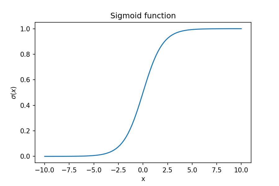
Over most of the range of the sigmoid function, the value is either 0 or 1, which is why this function is particularly suitable for a binary classifier. When we are fitting a model, we would like to find the coefficients that best fit the data. Including these coefficients results in an equation of this form:
where
is the probability of observation
being in class 1. The coefficients
and
determine the shape of the function and are what we are trying to fit
when we model our data. When we know the coefficients, we can make a
prediction of the class for an observation
.
Follow Along
# Import seaborn and load the data
import seaborn as sns

geyser = sns.load_dataset("geyser")

# Choose one feature - we'll use the duration
x = geyser['duration']

# Import the label encoder and encode the 'kind' column
from sklearn.preprocessing import LabelEncoder
le = LabelEncoder()

# Create a new column with 0=long and 1=short class labels
geyser['kind_binary'] = le.fit_transform(geyser['kind'])
display(geyser.head())

# Assign the target variable to y
y = geyser['kind_binary']
| duration | waiting | kind | kind_binary | |
|---|---|---|---|---|
| 0 | 3.600 | 79 | long | 0 |
| 1 | 1.800 | 54 | short | 1 |
| 2 | 3.333 | 74 | long | 0 |
| 3 | 2.283 | 62 | short | 1 |
| 4 | 4.533 | 85 | long | 0 |
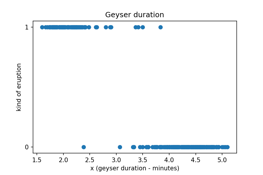
We now have a DataFrame with a column encoded with two classes: long=0
and short=1. Let's plot the duration column against the
binary classes we just created.
# Plot the data for 'duration'
plt.scatter(x, y)
plt.yticks([0, 1])
plt.xlabel('x (geyser duration - minutes)'); plt.ylabel('kind of eruption')
plt.title('Geyser duration')

plt.show()
Now, let's use the sigmoid function with coefficients from a model that fits the above data. We'll get to this step in the next objective so for now let's just focus on what the coefficient means and how to interpret the result. We'll assign the coefficients to variables and then plot the new function on our data above.
# Assign coefficient from previously fit model
beta_0 = 11.32
beta_1 = -3.65

# Define the sigmoid with the coefficients
def sigmoid_beta(x, beta_0, beta_1):
    exp = beta_0 + beta_1*x
    return 1 / (1 + np.e**(-exp))

x_model_plot = np.linspace(1, 6, 100)
y_model = sigmoid_beta(x_model_plot, beta_0, beta_1)

# Plot the function generated above
plt.scatter(x, y)
plt.plot(x_model_plot, y_model, color='green', label='model')
plt.xlabel('x (geyser duration - minutes)'); plt.ylabel('P( y=1 )')
plt.legend()
plt.title('Geyser eruption with model')

plt.show()
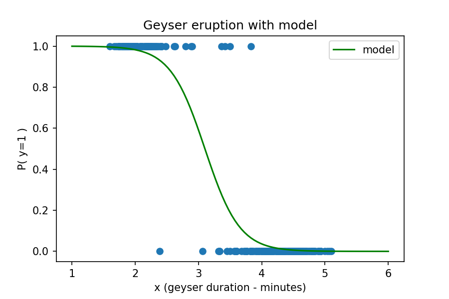
Now let's use our function with the model parameters to make and interpret a prediction. We'll pretend that we have visited the geyser site and viewed an eruption, which we timed to be 3.25 minutes. Which class would this eruption belong to and with what probability?
We know from the equation above that the probability is for the observation to belong to class=1 (short eruption). Plugging in the values for x (3.25 minutes) along with the coefficients gives us the following equation:
We interpret this result to mean that the probability of belonging to class=1 (short) is 37%. The probability of the observation belonging to class=0 (long) is 100%-37% = 63%. Our model predicts that an eruption with a duration of 3.25 minutes would belong to the long class of eruption.
Challenge
Using the same geyser data set in the example above, plot the
waiting
column along with the binary class we assigned above
(kind_binary). Sketch out the shape of the sigmoid
function that would best fit the data.
Additional Resources
Objective 04 - Use scikit learn to fit and interpret logistic regression models
Overview
So far, we've looked at the function and coefficients used to fit a
logistic regression. In this objective we're going to go more into
detail about how to use the scikit learn
LogisticRegression predictor. We'll also cover how to fit
this model using the two features in the dataset and how to interpret
these results.
Follow Along
Let's load the geyser data set we used earlier, and go through the steps to fit a logistic regression model.
# Import seaborn and load the data
import seaborn as sns

geyser = sns.load_dataset("geyser")

# Convert target labels to 0 or 1

# Import the label encoder and instantiate
from sklearn.preprocessing import LabelEncoder
le = LabelEncoder()

# Create a new column with 0=long and 1=short class labels
geyser['kind_binary'] = le.fit_transform(geyser['kind'])
display(geyser.head())
| duration | waiting | kind | kind_binary | |
|---|---|---|---|---|
| 0 | 3.600 | 79 | long | 0 |
| 1 | 1.800 | 54 | short | 1 |
| 2 | 3.333 | 74 | long | 0 |
| 3 | 2.283 | 62 | short | 1 |
| 4 | 4.533 | 85 | long | 0 |
Now that we have our geyser class encoded, we can follow the usual
model fitting procedure. First, we create the feature matrix and
target array. Then we import the
LogisticRegression model, instantiate the predictor
class, and fit the model.
# Import logistic regression predictor
from sklearn.linear_model import LogisticRegression

# Prepare the feature (we'll begin with one feature)
import numpy as np

x = geyser['duration']
X = np.array(x)[:, np.newaxis]

# Assign the target variable to y
y = geyser['kind_binary']

# Fit the model using the default parameters
model = LogisticRegression()
model.fit(X, y)LogisticRegression()# Import the cross validation method
from sklearn.model_selection import cross_val_score
# Implement a cross-validation with k=5
print(cross_val_score(model, X, y, cv=5))
# Calculate the mean of the cross-validation scores
score_mean = cross_val_score(model, X, y, cv=5).mean()
print('The mean CV score is: ', score_mean)
[0.94545455 1.         1.         0.94444444 1.        ]
The mean CV score is:  0.977979797979798
This model is pretty accurate. If we remember from earlier in this module, our baseline accuracy was 63%. We've improved over the baseline by a significant amount.
Now, how much can we improve our model by using an additional feature
in fitting our model? We still have the waiting column
which is the amount of time that passes between eruptions. Let's add
that feature to the feature matrix, fit the model, and calculate the
cross-validation score.
# Create new feature matrix
features = ['duration', 'waiting']
X_two = geyser[features]

# Fit the model using the default parameters
model_two = LogisticRegression()
model_two.fit(X_two, y)

# Implement a cross-validation with k=5
print(cross_val_score(model_two, X_two, y, cv=5))

# Calculate the mean of the cross-validation scores
score_mean = cross_val_score(model_two, X_two, y, cv=5).mean()
print('The mean CV score is (two features): ', score_mean)
[1. 1. 1. 1. 1.]
The mean CV score is (two features):  1.0
TThe accuracy is perfect for this model. This is likely because the two classes have a very clear division. It's important to remember that not all data sets will be so easy to model with such accurate results!
Challenge
For this challenge, try to plot the two features on the same plot. So instead of a plot with the feature on the x-axis and the class on the y axis, plot one feature on each axis. Are the two classes distinct as visualized on the plot? If you use two different colors for the classes, there should be a clear division between them. Think about where you would draw the decision boundary.
Additional Resources
Objective 05 - Use scikit-learn pipelines
Overview
In previous modules, we processed our data and fit the model in separate steps. We completed each step separately in order to better understand the process. Sometimes there are a number of steps needed before the model is fit, including encoding, imputing missing values, standardizing, and normalizing variables.
Each of these steps also needs to be applied to both the training data and the testing data, making for many extra lines of code. In order to streamline the preprocessing and model fitting, we can use a scikit-learn method called a pipeline.
Pipeline
The scikit-learn pipeline is used to apply a list of preprocessing steps and the final estimator, all in one step. Another important advantage of using a pipeline is that the same steps can be applied to data in the same fold of a cross-validation.
Follow Along
There are two ways to use the scikit-learn pipeline tool. The main one
is to use sklearn.pipeline.Pipeline(), where each step in
the pipeline is tuple of the name and transformer or estimator. For
example, creating a pipeline using the StandardScaler and
the SVC estimator would result in
pipe = Pipeline([('scaler', StandardScaler()), ('svc',
            SVC())])
.
An easier implementation is to use the
sklearn.pipeline.make_pipeline() convenience function.
Instead of a list of tuples, this function just accepts the
transformers and estimators; the names are set to the lowercase of
their types automatically. An example of this function is:
make_pipe = make_pipeline(StandardScaler(), SVC()).
Implement a Pipeline
Going back to our well-loved penguin data set, we're going to use a pipeline to pre-process and fit a model to predict which class a penguin belongs to (male or female). Let's load in the data and discuss each step as we work through the pipeline.
# Load in the data!

import pandas as pd
import seaborn as sns

penguins = sns.load_dataset("penguins")

# Remove NaNs and nulls
penguins.dropna(inplace=True)

display(penguins.head())
| species | island | bill_length_mm | bill_depth_mm | flipper_length_mm | body_mass_g | sex | |
|---|---|---|---|---|---|---|---|
| 0 | Adelie | Torgersen | 39.1 | 18.7 | 181.0 | 3750.0 | Male |
| 1 | Adelie | Torgersen | 39.5 | 17.4 | 186.0 | 3800.0 | Female |
| 2 | Adelie | Torgersen | 40.3 | 18.0 | 195.0 | 3250.0 | Female |
| 3 | Adelie | Torgersen | 36.7 | 19.3 | 193.0 | 3450.0 | Female |
| 4 | Adelie | Torgersen | 39.3 | 20.6 | 190.0 | 3650.0 | Male |
We have a few features to choose from to fit our model. Let's use
species, bill_length_mm,
bill_depth_mm, flipper_length_mm, and
body_mass_g. Our target will be the sex of
the penguin.
Feature Matrix
We have one categorical feature (species) and four
numeric features. We'll use one-hot encoding to transform the
species column into three one-hot encoded columns. And
the target array (sex) will also be encoded with the
label encoder. That won't be part of the preprocessing of the
features; we'll do that separately before we apply our pipeline steps
and fit the model.
In the following code we will use the
OneHotEncoder() method for the
species column. When we use this method we also need to
use the ColumnTransformer() method to apply the one-hot
encoder to our specified column.
# Imports!
from sklearn.compose import ColumnTransformer
from sklearn.pipeline import Pipeline
from sklearn.preprocessing import OneHotEncoder
from sklearn.linear_model import LogisticRegression
from sklearn.model_selection import train_test_split

# Set-up the one-hot encoder method
categorical_features = ['species']
categorical_transformer = Pipeline(steps=[('onehot', OneHotEncoder())])

# Set up our preprocessor/column transformer
preprocessor = ColumnTransformer(
    transformers=[
        ('cat', categorical_transformer, categorical_features)])

# Append classifier to preprocessing pipeline.
# Now we have a full prediction pipeline.
clf = Pipeline(steps=[('preprocessor', preprocessor),
                      ('classifier', LogisticRegression())])
Feature Matrix and Target Array
We need to select our features and encode our target array. These steps are pretty simple and do not need to be part of the preprocessing pipeline.
# Select features
features = ['species', 'bill_length_mm', 'bill_depth_mm', 'flipper_length_mm', 'body_mass_g']
X = penguins[features]

# Encode the 'sex' column
from sklearn import preprocessing
le = preprocessing.LabelEncoder()
penguins['sex_encode'] = le.fit_transform(penguins['sex'])

# Set target array
y = penguins['sex_encode']
Now that we have our feature matrix (still in categorical form) and a label encoded target array, we can apply the pipeline and actually fit the model!
# Apply the pipeline

# Separate into training and testing sets
X_train, X_test, y_train, y_test = train_test_split(X, y, test_size=0.25)

# Fit the model with our logistic regression classifier
clf.fit(X_train, y_train)
print("model score: %.3f" % clf.score(X_test, y_test))
model score: 0.440
With just one line of code we one-hot encoded our specified features and fit a logistic regression model to our data. Using the pipeline allowed us to apply the same transformations to our training and testing data sets without having to repeat those steps.
Challenge
Using the above code example, let's see if you can improve the model
score. In the LogisticRegression() part, try to change
the inverse of regularization strength parameter C. You
could also adjust the number of features used in the model to see how
that affects the accuracy.
Additional Resources
RESOURCE - Local Installation (Windows)
Common Command Prompt Commands
Video: Common Command Prompt CommandsYou should be familiar with the following commands:
dircdmkdir
Install and Configure Git
Video: Installing GitInstallation
Download the latest 64-bit version of git for Windows.
Once the installer opens, select the following options from the prompts:
-
Choosing the default editor used by Git
Choose anything other than Vim (for example, VS Code) -
Adjusting your PATH enviroment
Choose “Git from the command line and also from 3rd-party software” -
Choosing HTTP transport backend
Choose “Use the OpenSSL library” -
Configuring the line endings conversions
Choose “Checkout Windows-style, commit Unix-style line endings” -
Configuring the terminal emulator to use with Git Bash
Choose “Use MinTYY” -
Choose the default behavoir of git pull
Choose “Default" (fast-forward or merge) -
Choose a credential helper
Choose “Git Credential Manager” -
Configuring extra options
Check the box for “Enable file system caching” -
Configuring experimental options
Make sure that no boxes are checked
Configuration
In order to work with the BloomTech curriculum repos, you need to configure git on your machine. Open up the Command Prompt, and type out these commands, following each with ENTER.
While you can use any username, you should use the username that's associated with your GitHub profile.
git config --global user.name <your username>Be sure that this email is the same one associated with your GitHub account.
git config --global user.email <your email address>If you'd like to use VS Code to write your commit messages:
git config --global core.editor "code --wait"And to make sure there are no conflicts with line endings:
git config --global core.autocrlf trueInstall Python
Video: Installing Python 64 bit (Windows 10)Download the latest version of Python for Windows. Note: It is very important that you download the Windows 64-bit executable installer.
Once the installer has opened, select the Add Python to PATH box and click Customize installation. Then select the following options from the prompts:
-
Optional Features
Check all the boxes. Make sure that the “pip” option is selected. -
Advanced Options
Select “Associate files with Python,” “Create shortcuts for installed applications,” and “Add Python to environment variables. This last option is especially important.
Install pipenv
Video: Installing pipenv (Windows 10)Open the command prompt and enter:
pip install pipenv
To check that pipenv has been installed, close the Command Prompt and
reopen. Then enter pipenv. If you see some help prompts,
you're all set!
Build a Virtual Enviroment
Build Enviroment on the Fly
Video: Building a Virtual Environment with pipenv
In the Terminal, use the cd command to navigate to the
folder where you want to build your environment. For example,
cd Documents/GitHub/testenvOnce you're in the correct directory, execute the command:
pipenv shellYou'll know that your virtual environment is active if your command line starts with the name of the environment in parentheses.
(testenv) <...> %
Use pipenv install <packages> to install the
packages that you'll use for the project, separated by spaces. For
example,
pipenv install pandas sklearn matplotlib notebook
You can also specify package versions using ==. For
example, pipenv install numpy==1.17.* would install
version 1.17 of numpy.
Note that if you want to use Jupyter notebooks, you always need to
install the notebook package.
Build Enviroment from requirements.txt File
Video: Building a Virtual Environment from a requirements.txt file
In the Terminal, use the cd command to navigate to the
folder where the requirements.txt file is located. For
example,
cd Documents/GitHub/testenvOnce you're in the correct directory, execute the command:
pipenv shell
Once your virutal enviroment is activated, use the following command
to install all the dependencies listed in the
requirements.txt file:
pipenv install -r requirements.txtRESOURCE - Local Installation (mac)
Before You Begin
- Make sure you're running the latest version of the the MacOS (Catalina, 10.15 or later).
- Make sure that your default shell in the terminal is z-shell.
Common Commands
You should be familiar with the following terminal commands:
- pwd
- cd
- ls
- mkdir
- clear
- nano
Installation
Install Xcode
In order to work locally on your Mac, you need to install Python 3 and pip3 on your machine. Fortunately, both of these come as part of Apple's Xcode. If you haven't already installed Xcode, open the Terminal and enter the following command:
xcode-select --installA popup window will appear. Click Install, and accept the user agreement.
To make sure that the latest version of pip3 has been installed, enter:
pip3 install --upgrade pip --userInstall pipenv
Once, pip3 is installed, you can use it to install pipenv:
pip3 install pipenv --userDuring installation, you may get a warning that looks something like this:
WARNING: The script virtualenv-clone is installed in 'Users/<your_username>/Library/Python/3.7/bin' which is not on PATHNote that the name of your path will a little look different: Your username will appear after User/, and you might have a different version number after Python/.
You will need to use this path later in the installation, so copy the Users/<your_username>/Library/Python/3.7/bin text and paste it somewhere where you can access it later.
Below the warning message, you should see a message saying that pipenv has been successfully installed.
Add Directory to Your PATH
Note: You only need to do this step if you got the warning above.
You now need to create a file named .zshrc that has this new path information. One way to do this is to use the program nano. In the terminal, enter:
nano ~/.zshrcThis will turn the terminal into a text editor. Go back to the path you copied during the last step and use it to write the following line:
export PATH="/Users/<your_username>/Library/Python/3.7/bin:$PATH"Make sure to insert your path after the " character, and then add :$PATH" to the end. There should be no spaces in this text.
Hit Ctrl+o then enter to save the file. Then Ctrl+x to quit.
Finally, quit the terminal (be sure to quit the program, not just close the window).
Confirm Installation
Reopen the terminal and enter the command pipenv. If the command line gives a list of options, then the install was successful!
Configure Git
In order to work with the BloomTech curriculum repos, you need to configure Git on your machine. Open up the Terminal, and type out the these commands, following each with ENTER.
While you can use any username, you should use the username that's associated with your GitHub profile.
git config --global user.name <your username>Be sure that this email is the same one associated with your GitHub account.
git config --global user.email <your email address>If you'd like to continue using nano to write commit messages, use:
git config --global core.editor "nano"Alternatively, you can use VS Code:
git config --global core.editor "code --wait"Build a Virtual Enviroment
Build Environment on the Fly
Video: Building a Virtual Environment from a requirements.txt fileIn the Terminal, use the cd command to navigate to the folder where you want to build your environment. For example,
cd Documents/GitHub/testenvOnce you're in the correct directory, execute the command:
pipenv shellYou'll know that your virtual environment is active if your command line starts with the name of the environment in parentheses.
(testenv) <...> %
Use pipenv install <packages> to install the
packages that you'll use for the project, separated by spaces. For
example,
pipenv install pandas sklearn matplotlib notebook
You can also specify package versions using ==. For example,
pipenv install numpy==1.17.* would install version 1.17
of numpy.
Note that if you want to use Jupyter notebooks, you always need to install the notebook package.
Build Enviroment from requirements.txt File
Video: Building a Virtual Environment from a requirements.txt fileIn the Terminal, use the cd command to navigate to the folder where the requirements.txt file is located. For example,
cd Documents/GitHub/testenvOnce you're in the correct directory, execute the command:
pipenv shellOnce your virtual environment is activated, use the following command to install all the dependencies listed in the requirements.txt file:
pipenv install -r requirements.txtGuided Project
Open JDS_SHR_214_guided_project_notes.ipynb in the GitHub repository below to follow along with the guided project:
Guided Project Video
Module Assignment
Complete the Module 4 assignment to practice logistic regression techniques you've learned.
Assignment Solution Video
Resources
Documentation and Tutorials
- Scikit-learn: train_test_split
- Scikit-learn: LogisticRegression
- Scikit-learn: Pipelines
- Scikit-learn: Classification Metrics