Module 3: Ridge Regression
Module Overview
In this module, you will build on your regression knowledge with ridge regression. You'll learn about one-hot encoding, feature selection, and how regularization can improve model performance. These techniques will help you handle categorical variables and build more effective models with many features.
Learning Objectives
- Implement one-hot encoding of categorical features
- Implement a univariate feature selection process
- Express and explain the intuition and interpretation of ridge regression
- Use sklearn to fit and interpret ridge regression models
Objective 01 - Implement one-hot encoding of categorical features
Overview
In the previous two modules, we focused only on numerical features. In the penguin data set however, there were also several other features like biological sex, penguin species, and island of origin. We did not use these non-numeric columns - but what if we had wanted add those features while building the model?
This type of data, known as categorical data, is composed of specific values that belong to a finite set of categories or classes. For example, the column labeled "sex" has two values: male and female. This is a specific type of data called a binary variable. It would be a simple process to convert the "male" values to 0 and the "female" values to 1. We would then have a numeric vector that can be used as input for a model.
What if we had a column that had more than two categories? We could do something called "ordinal encoding" where we assign an integer to each class. For example, there could be other values in the "sex" column to indicate an indeterminate value or just unknown. We could assign these values to a class equal to '3'. Then, our ordinal encoding would be 1, 2, 3 (female, male, unknown/other).
There is a problem with this method: it implies some ranking of the categories. How we assigned the ordinal values was random: we could have assigned 'unknown'= 1, 'female'= 2, and 'male'= 3. So the ordering of the classes doesn't have any meaning.
One-hot encoding
To get around this "ranking" issue we can use one-hot encoding. Instead of using ordinal integers we can create new feature vectors by encoding with a 0 or 1. Using the above example, we could take the single "sex" column that contains three categories and convert it to three columns, with values of '0' or '1'. The following tables show this more clearly.
Original feature column
| sex |
|---|
| male |
| male |
| female |
| other |
| male |
| female |
One-hot encoded column
| male | female | other |
|---|---|---|
| 1 | 0 | 0 |
| 1 | 0 | 0 |
| 0 | 1 | 0 |
| 0 | 0 | 1 |
| 1 | 0 | 0 |
| 0 | 1 | 0 |
We now have three feature vectors, each with a '1' corresponding to when that class is present. Each value can't belong to more than one class at a time, so the cell that is "on" (has a '1') is the "hot" cell.
Follow Along
We're going to work through an example using scikit-learn utilities to one-hot encode the "species" column in the penguin data set. Let's load the data, and look at the data frame and the number of classes in the species column.
import seaborn as sns

# Bring in the penguins!
penguins = sns.load_dataset("penguins")
display(penguins.head())

# Find the number of classes in species
penguins['species'].unique()
| species | island | bill_length_mm | bill_depth_mm | flipper_length_mm | body_mass_g | sex | |
|---|---|---|---|---|---|---|---|
| 0 | Adelie | Torgersen | 39.1 | 18.7 | 181.0 | 3750.0 | Male |
| 1 | Adelie | Torgersen | 39.5 | 17.4 | 186.0 | 3800.0 | Female |
| 2 | Adelie | Torgersen | 40.3 | 18.0 | 195.0 | 3250.0 | Female |
| 3 | Adelie | Torgersen | NaN | NaN | NaN | NaN | NaN |
| 4 | Adelie | Torgersen | 36.7 | 19.3 | 193.0 | 3450.0 | Female |
array(['Adelie', 'Chinstrap', 'Gentoo'], dtype=object)
We have three species listed, which is a good number of categories to
demonstrate with. The species values are string objects, which is
accepted as input to the
sklearn.preprocessing.OneHotEncoder()
transformer. We need to reshape the array so that it's 2D using the
np.newaxis method as before.
# Imports
import numpy as np

# Select and reshape input array
species = penguins.species[:, np.newaxis]

# Import the encoder
from sklearn.preprocessing import OneHotEncoder

# Instantiate the encoder as an object
enc = OneHotEncoder(sparse=False)

# Use the fit_transform method (2 steps in 1)
onehot = enc.fit_transform(species)

# Display every 25th row
onehot[::25]
array([[1., 0., 0.],
       [1., 0., 0.],
       [1., 0., 0.],
       [1., 0., 0.],
       [1., 0., 0.],
       [1., 0., 0.],
       [1., 0., 0.],
       [0., 1., 0.],
       [0., 1., 0.],
       [0., 0., 1.],
       [0., 0., 1.],
       [0., 0., 1.],
       [0., 0., 1.],
       [0., 0., 1.]])
The species column values, containing three classes, is now an array of three vectors. In each of the columns we can see there is only one "hot" cell ('1') and the rest are zeros.
Challenge
In the penguins data set there is another column ("island") that can be one-hot encoded. Following the same process as above, one-hot encode this column. As a stretch goal, you can concatenate the one-hot encoded array with the original DataFrame. This will be useful when we want to use the dataset in a model where you need to provide a single feature matrix; each one-hot encoded column will be treated as a feature.
Additional Resources
Objective 02 - Implement a univariate feature selection process
Overview
We've discussed the concepts of feature engineering and feature selection in the earlier Sprints. Now that we are becoming more familiar with a variety of machine learning topics, it's time to come back to this important concept and learn how to select the features we would like to include in our models.
In the previous module we discussed the concepts of underfitting-overfitting models and the relationship to the bias-variance trade-off. We can expand this concept and focus on how the number of features we use in a model impacts the results. For example, consider the case where we are using a complicated model with a lot of features. When we look at how the model performs on the testing set, we might decide it's not a good fit and find a need to make the model simpler.
One method to reduce model complexity is by using fewer features. This decreases the number of parameters that need to be fit by the model and increases the chance that the model will generalize well. So, how do we determine which features, and how many, to keep in our model?
One of the more popular approaches to feature selection is the univariate feature selection process. The name originates from the process of looking at each feature individually and measuring the strength of its relationship with the target feature. For a linear regression, we would take each independent feature and separately measure the strength of the linear correlation with the dependent variable.
We'll work through an example with the penguin data set (yes, again - it's a nice data set to work on!).
Follow Along
We remember from the penguin data set that we have six features and one target. In our uses we have been using the numeric features to predict the body mass of the penguins. We're going to continue with the numeric features for this next example.
# Import pandas and seaborn
import pandas as pd
import numpy as np
import seaborn as sns

# Load the data into a DataFrame
penguins = sns.load_dataset("penguins")

# Drop NaNs
penguins.dropna(inplace=True)

# Create the features matrix
features = ['bill_length_mm', 'bill_depth_mm', 'flipper_length_mm']
X = penguins[features]

# Create the target array
y = penguins['body_mass_g']

# Import the train_test_split utility
from sklearn.model_selection import train_test_split

# Create the training and test sets
X_train, X_test, y_train, y_test = train_test_split(
    X, y, test_size=0.2, random_state=42)
Using SelectKBest
The utility we're using to select the best features is the
SelectKBest method from the
sklearn.feature_selection module. The name of the method
makes it easier to remember what it does: select the k best features
where k is an integer.
# Import the feature selector utility
from sklearn.feature_selection import SelectKBest, f_regression

# Create the selector object with the best k=1 features
selector = SelectKBest(score_func=f_regression, k=1)

# Run the selector on the training data
X_train_selected = selector.fit_transform(X_train, y_train)

# Find the features that was selected
selected_mask = selector.get_support()
all_features = X_train.columns
selected_feature = all_features[selected_mask]

print('The selected feature: ', selected_feature[0])
The selected feature: flipper_length_mmThe flipper length seems to be the best feature to include when trying to predict the penguin's body mass.
Challenge
We only selected the single best feature; try the same process as
above but set k=2 and see which are the two best
features. You can also use the one-hot encoded feature columns from
the previous objective as additional features. Are any of those
columns a good feature when trying to predict body mass?
Additional Resources
Objective 03 - Express and explain the intuition and interpretation of ridge regression
Overview
When we are training a model, simple is usually better. With fewer parameters to determine, the model is easier to interpret. Also, with too many parameters there is a chance the model will fit the training data well but won't generalize to new data. This objective will focus on a specific type of regularization called ridge regression.
Regularization
The concept of regularization is to reduce variance in a model with a "shrinkage" penalty. A more formal definition of regularization is to add information or bias to prevent overfitting. In regression, there are two common types of regularization: ridge regression and lasso. Ridge regression uses a penalty where the tuning parameter is multiplied by the squared sum of all coefficients (L2). Lasso regression is similar, but the penalty is a tuning parameter multiplied by the sum of the absolute values of all the coefficients (L1).
Ridge Regression
A regression model determines the parameters that minimize the residual sum of squares (RSS). The basis of ridge regression is to minimize the residual sum of squares (RSS) plus some penalty multiplied by the sum of the squares of the coefficients. The larger the penalty, the more the parameters are penalized, especially large parameters. The penalty or tuning parameter is called both lambda and alpha; lambda means something in Python already, so we'll use alpha for this discussion.
Note: the term "ridge" refers to the shape of the function we are trying to minimize. We turn a ridge into a peak where the parameters that minimize the RSS plus the penalty term are located at this peak.
Standardization
Another consideration when using any type of regularization technique is standardization. If the variables are on different scales, the larger variable will have a different contribution to the penalized terms. For example, if we were predicting weight from height, if height is in meters, a change of one unit will be a large change in weight. If height is in a smaller unit like centimeters, a unit change will be a much smaller change in weight.
Follow Along
Now that we have gone over the concepts of regularization and ridge regression, let's look at the math illustrated with a few plots to help us understand the concept better.
Sum of Squares
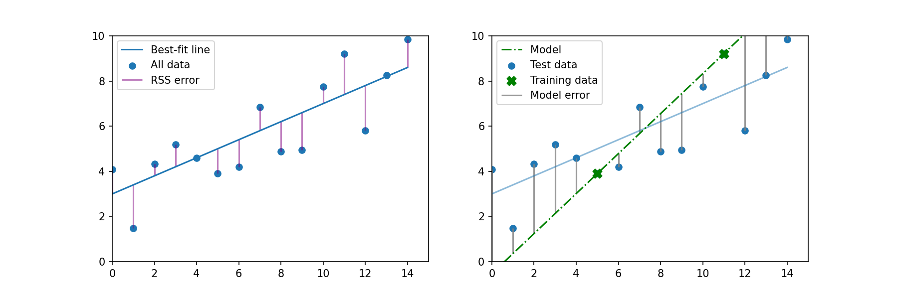
When we fit a linear regression, we want to find the parameters (slope and intercept) that minimize the sum of the squares of the distance from each data point to the best-fit line. In the plot below on the left, the sum of the errors is shown by the solid magenta line. Now let's take two of these data points and call them our "training data" (plot on the right). With two points, we can fit a perfect line which has no error. But the RSS error has increased, which is indicated by the gray "model error" line in the plot on the right.
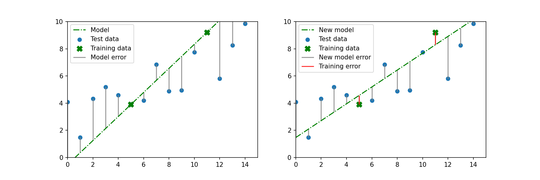
With ridge regression, we want to introduce a small amount of bias in the training data. In other words, we don't want the line to fit these two training points perfectly. With this new line there is a small amount of error (red lines). With this new, slightly biased model, the RSS for the rest of the data has decreased.
Additional Resources
Objective 04 - Use sklearn to fit and interpret ridge regression models
Overview
In the previous objective, we looked at a simple example of how the introduction of bias reduces the variance in a model. Now, we're going to implement three different models: a linear regression, a linear regression with a number of polynomial features, and a ridge regression.
Follow Along
Let's look at our examples. First, we'll generate a data set to practice with. Let's pretend that this data represents the number of ice cream cones sold according to the hour after the shop opened. We would like to fit this data to predict how much ice cream will be sold later in the day.
# Generate the practice data set
import numpy as np

np.random.seed(15)
x = 5 * np.random.rand(50)
y = abs(0.5*np.sin(x) + 0.5 * np.random.rand(50))*10

# Create the feature matrix
X = x[:, np.newaxis]

# Fit a linear regression model
from sklearn.linear_model import LinearRegression
model = LinearRegression()
model.fit(X, y)

# Create the data for the model (best-fit line)
xfit = np.linspace(0, 5, 1000)
Xfit = xfit[:, np.newaxis]
yfit = model.predict(Xfit)
# Fit a linear regression with polynomial features
from sklearn.preprocessing import PolynomialFeatures
from sklearn.pipeline import make_pipeline
poly_model = make_pipeline(PolynomialFeatures(15),
LinearRegression())
# Create the data for the model (best-fit line)
poly_model.fit(x[:, np.newaxis], y)
yfit_poly = poly_model.predict(xfit[:, np.newaxis])
# Fit a ridge regression with polynomial features
from sklearn.linear_model import Ridge
from sklearn.preprocessing import StandardScaler

ridge_model = make_pipeline(PolynomialFeatures(15),
                            StandardScaler(),
                            Ridge(alpha = 0.05))

ridge_model.fit(x[:, np.newaxis], y)

# Create the data for the model (best-fit line)
yfit_ridge = ridge_model.predict(xfit[:, np.newaxis])
Now we'll create a plot with our practice data and all three models.
import matplotlib.pyplot as plt

fig, ax = plt.subplots(figsize=(10,5))
ax.scatter(x,y)

ax.plot(xfit, yfit, linestyle='--', label='linear regression')
ax.plot(xfit, yfit_poly, linestyle = '-.', label='linear regression (polynomial)')
ax.plot(xfit, yfit_ridge, label='ridge regression')

ax.set_ylim([0, 10])

ax.set_xlabel('Hours after opening')
ax.set_ylabel('Ice cream sales')
ax.legend()

plt.show()
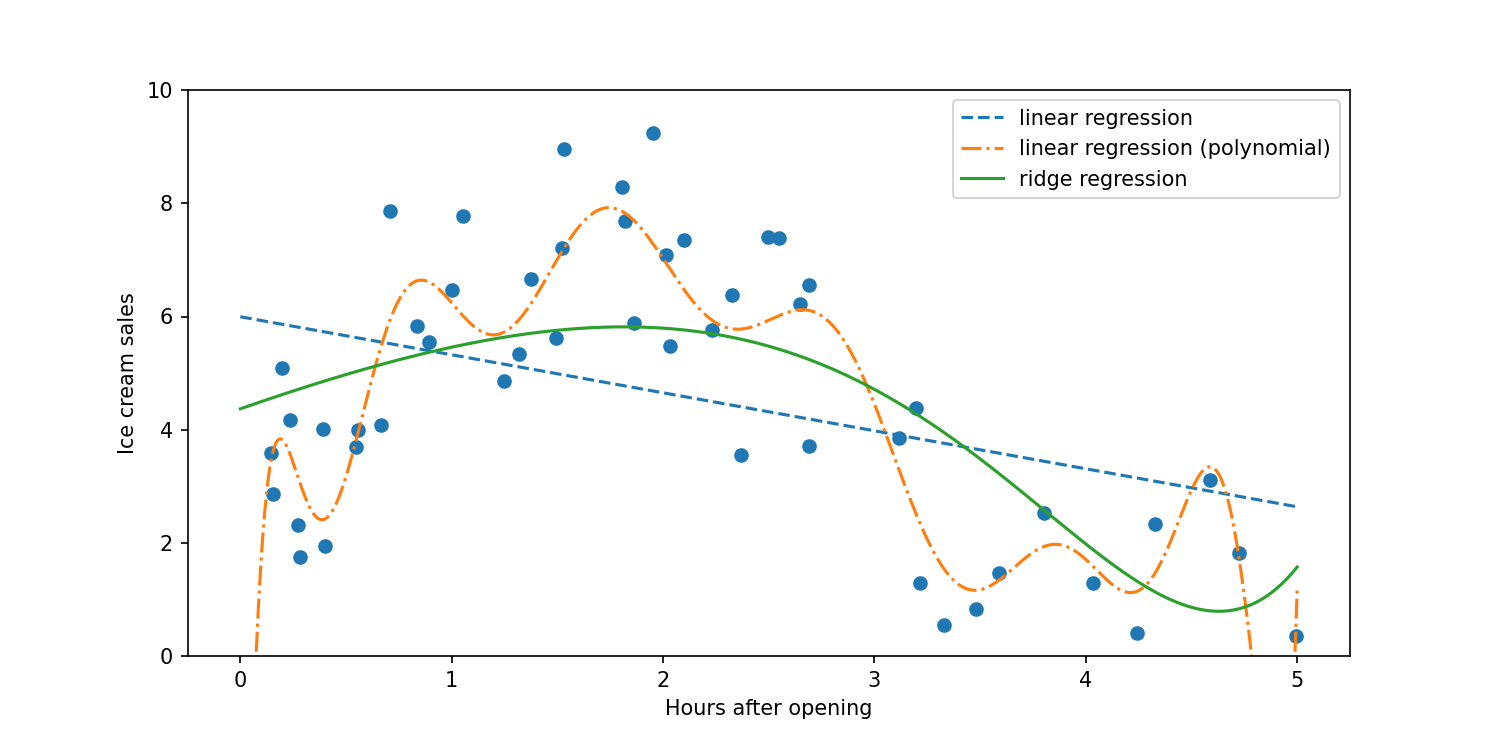
In the above plot, we can see that the linear regression with a number of polynomial features (15) tries to fit all the little increases and decreases in the data set. We wouldn't want to try to predict what future ice cream sales would look like with the orange dash-dot line. The model fit by using ridge regression (solid green line) is a better fit to the data and captures the decrease in sales 4-5 hours after opening. Even though the ridge regression model uses the same degree polynomial as the orange dash-dot line, the parameters are penalized by the ridge regression alpha parameter.
Challenge
With the code example above, try selecting a different value for alpha. The larger the value, the more the parameters are penalized and the less likely they are to affect the model. You can also experiment and set alpha=0 and see what the resulting model is.
Additional Resources
Guided Project
Open JDS_SHR_213_guided_project_notes.ipynb in the GitHub repository below to follow along with the guided project:
Guided Project Video
Module Assignment
Complete the Module 3 assignment to practice ridge regression techniques you've learned.
Assignment Solution Video
Resources
Documentation and Tutorials
- Scikit-learn: OneHotEncoder
- Scikit-learn: Feature Selection
- Scikit-learn: Ridge Regression
- Scikit-learn: Ridge Class