Module 1: Linear Regression 1
Module Overview
In this module, you will learn the fundamentals of linear regression. You'll start with simple baseline models, implement linear regression using scikit-learn, and understand how to interpret model coefficients.
Learning Objectives
- Determine baseline for Regression
- Fit a Simple Linear Regression model using scikit learn
- Explain Linear Regression Coefficients
Objective 01 - Begin with baselines for regression
Overview
In this module we're going to be focusing on regression. Regression analysis is used to determine the relationship between a continuous dependent variable and an independent variable(s). In machine learning, regression is often used to make predictions. We're going to start by introducing linear regression with continuous variables and work through using scikit-learn to fit a linear regression model to some practice datasets.
Before we practice model fitting using regression, we need to understand the concept of a baseline.
Baselines
A common definition of a baseline is a starting point from which to make comparisons. If we fit a model to our data, we need to have a starting place to compare our results to.
There are different metrics we can use as our baseline. Some that we'll consider in this module are: using a "rule of thumb" (using previous knowledge or commonly known information), descriptive statistics (such as the mean, minimum, or maximum or the variable), and fitting a simple model (such as a linear regression that can serve as a baseline for a more complicated model).
Using an example dataset, let's look at how to determine the type of baseline that is appropriate for the data and the type of model we would like to fit.
Follow Along
For this next exercise, we're going to step into the role of a penguin researcher. For our research, we'd like to be able to predict the weight of a penguin (the mass) based on the length of the flippers (these are analogous to a bird's wings). The length of a flipper is easier to observe than other less obvious physical characteristics and so we'd like to use it to easily predict the penguin's weight.
Baseline
Since we're serving as (temporary) penguin researchers, we have some experience with judging the weight of a penguin by the flipper length. We know that on average, for about every 20 mm increase in flipper length, the weight of the penguin increases by about 1000 g (1 kg). One of our penguins has a flipper length of 220 mm and we also know his weight is 5000 g. We observe another penguin to have a flipper length of 190 mm; what is the approximate weight of this second penguin? We know we have an increase of 1000g/20mm. The second penguin's flippers are 30mm shorter so the weight would be 5000g - 1500g = 3500g.
We just used a baseline (1000g/20mm) and made a prediction based on that starting point.
Check the Baseline
As penguin researchers, we have some data available to us. The next step is to plot our data and then do a simple regression to fit a line; we'll expand on this step in the next objective.
The seaborn plotting library has conveniently made the penguin data available. Once we import seaborn, we can easily load the dataset into a DataFrame.
# Import seaborn and matplotlib with the standard aliases
import seaborn as sns
import matplotlib.pyplot as plt

# Load the example penguins dataset
penguins = sns.load_dataset("penguins")

# Create a "regplot"
sns.regplot(x="flipper_length_mm", y="body_mass_g", data=penguins, fit_reg=True)

plt.show()
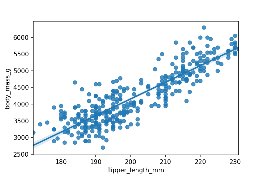
Because seaborn doesn't display the actual equation for the regression, we'll check our
answer the old-fashioned way by adding grid lines to the plot. You could also use the scikit-learn
linear regression estimator, which we'll work through later in the module.
# Plot the same data as above but with added lines for our "guess"
ax = sns.regplot(x="flipper_length_mm", y="body_mass_g", data=penguins, fit_reg=True)
plt.axvline(x=190, color='red', linewidth=0.75)
plt.axhline(y=3500, color='red', linewidth=0.75)

plt.show()
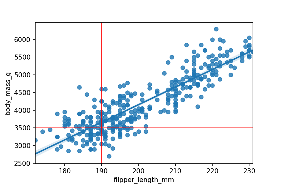
Where the lines intersect is what we guessed our penguin's weight to be, based on our prior knowledge of a general flipper length to weight ratio. The intersection is pretty close to the best-fit line (linear regression fit by seaborn) - our baseline guess wasn't too bad!
Challenge
Using the penguin data set, try selecting a different flipper length and then use the ratio of 1000g/20mm to predict the weight of the penguin. As a stretch goal, you can plot your guess using the same code as above, and see how well our baseline does.
Additional Resources
Objective 02 - Use scikit-learn for linear regression
Overview
In the previous objectives, we used seaborn to fit a simple linear regression to a dataset
containing
penguin weight and flipper lengths. In the example, we compared our baseline (the ratio of weight to
flipper length) to the actual best-line fit in the plot.
Throughout this unit we're going to be using the tools available in the scikit-learn library. Most likely you've already come across this library and even used some of the tools, either in Unit 1 or during your own learning.
Right now, we're going to work through an example using scikit-learn to fit a linear regression model, using the same dataset from the previous objective. While some of this material may be review, it's still important to go through each of the steps, both for practice and to address concepts that we might have missed.
Linear Regression
Before we get into how to use scikit-learn to fit a model, we'll do a quick review of linear regression and the associated coefficients. Linear regression fits a line to data where the equation of the line is given by
When we fit a line, we're trying to find the coefficients β and α. The parameter α is the intercept (when x = 0, the intercept is the y value) and β is the slope. The results of the model fit will return the slope and intercept.
When we fit a line, we're trying to find the coefficients and . The parameter is the intercept (when , the intercept is the value) and is the slope. The results of the model fit will return the slope and intercept.
In the next objective we'll focus more on the meaning of the coefficients. Right now the goal is to learn how to use the scikit-learn tool to fit a simple model.
Follow Along
The following steps show the same process you will follow with the scikit-learn API (application programming interface; how we interact with the many tools in the scikit-learn predictor) to fit many different types of models. The model type, model complexity, data type, and size of the data set will not affect the following steps:
Scikit-learn API
- Load the data set and "clean” if needed (not specifically part of scikit-learn but essential to the DS process)
- Create features and target(s) from the data
- Import the model and instantiate the class
- Fit the model
- Apply your model; use the model to predict new values
In the above process, the data loading, cleaning, and preparing for modeling can be done all at once before any of the other steps. Creating features and target(s) can also be completed right before you fit the model; the important thing to remember is to have the data in the correct form before fitting.
Load Data
As in the previous objective, we'll use the penguin data set available from the seaborn library. When we import seaborn, all of the associated datasets are included; we don't need to download any other data or load files from our local system.
We also need to make sure we remove any NaN values now. The model-fitting algorithm requires that we input clean data or data that is free of missing values.
# Import pandas and seaborn
import pandas as pd
import numpy as np
import seaborn as sns

# Load the data into a DataFrame
penguins = sns.load_dataset("penguins")

# Print the shape of the DataFrame
print('Shape of the dataset (before removing NaNs): ', penguins.shape)

# Drop NaNs
penguins.dropna(inplace=True)

# Print the shape of the DataFrame
print('Shape of the dataset (after removing NaNs): ', penguins.shape)

# Display the first five rows
display(penguins.head())
Shape of the dataset (before removing NaNs): (344, 7)
Shape of the dataset (after removing NaNs): (333, 7)| species | island | bill_length_mm | bill_depth_mm | flipper_length_mm | body_mass_g | sex | |
|---|---|---|---|---|---|---|---|
| 0 | Adelie | Torgersen | 39.1 | 18.7 | 181.0 | 3750.0 | Male |
| 1 | Adelie | Torgersen | 39.5 | 17.4 | 186.0 | 3800.0 | Female |
| 2 | Adelie | Torgersen | 40.3 | 18.0 | 195.0 | 3250.0 | Female |
| 3 | Adelie | Torgersen | 36.7 | 19.3 | 193.0 | 3450.0 | Female |
| 4 | Adelie | Torgersen | 39.3 | 20.6 | 190.0 | 3650.0 | Male |
Representing Data
In the previous Sprints, we discussed how organizing our data in a particular format, makes it easier to clean it for machine learning. Now we get to see the benefit of having such formatted data as we prepare to use it with scikit-learn.
In the above table, we have 333 rows of data (after filtering), where each row is an observation of
a
single penguin. The rows are sometimes called samples; think of each row as a sample of observations
about a penguin. We also have seven columns that correspond to the information that describes each
sample. In the columns we are describing the species, home island, and physical characters of our
samples (penguins). Features are often numeric like (body_mass_g,
flipper_length_mm) but not always.
The species, island, and sex columns are all described by string
variables.
Feature Matrix and Target Array
Before we can input our data into a scikit-learn model, we have to separate it into a feature matrix
and
target array. First, we need to decide what we're trying to predict from this dataset. We've already
fit
a simple linear regression model to the flipper_length_mm and body_mass_g
variables, so we'll continue with those two variables. We want to use the flipper length to predict
the weight of the penguin.
The
terminology we use is as follows: our feature (flipper length) will be used to predict the target
(weight).
For this simple linear regression example, we are only predicting one target variable; the target is an array with a length equal to the number of rows in the feature matrix.

In the following code, we'll create our feature matrix and target vector/array. It's customary to use a capital (uppercase) X, for the features, and a lowercase y, for the target vector. We'll add the name penguins to our variable names to make it easier to remember the data we are fitting.
# Create the feature matrix
X_penguins = penguins['flipper_length_mm']
print("The shape of the feature matrix: ", X_penguins.shape)

# Create the target array/vector
y_penguins = penguins['body_mass_g']
print("The shape of the target array/vector: ", y_penguins.shape)
The shape of the feature matrix: (333,)
The shape of the target array/vector: (333,)
We can see that these are both one-dimensional arrays of 333 elements, which is what we expected. Our data is now ready to be input in a scikit-learn model.
Scikit-learn Predictor
The scikit-learn predictor is the object that learns from the data. There is a standard process to follow to use the predictor object. Our example will be for a linear regression but we can apply these steps to any of the scikit-learn predictors (classification, regression, and clustering).
-
Import the model class
We already know we're trying to fit a linear model to our data, so we'll use a regression algorithm.from sklearn.linear_model import LinearRegression -
Instantiate the class
The term instantiate is a fancy way to say you are creating an instance of a class. We imported the predictor class but that's it; we need to create an instance of that class to actually do anything. With this step, we also determine the hyperparameters or model parameters we would like to use.To create an instance of LinearRegression() predictor, we use the following code:
# Import the predictor class
from sklearn.linear_model import LinearRegression

# Instantiate the class (with default parameters)
model = LinearRegression()

# Display the model parameters
model
LinearRegression()
The LinearRegression() predictor has four parameters that we can set. For now, let's use the default setting but you can read more about the parameters here.
-
Arrange data
Part of this step was already completed above, but all predictors require the feature matrix to be in the form of a two-dimensional matrix. We can reshape the one-dimensional array by adding a new axis with the np.newaxis function.# Ensure X_penguins is a NumPy array if it's a pandas Series if isinstance(X_penguins, pd.Series): X_penguins = X_penguins.to_numpy() # Display the shape of X_penguins print('Original features matrix: ', X_penguins.shape) # Add a new axis to create a column vector X_penguins_2D = X_penguins[:, np.newaxis] print(X_penguins_2D.shape)Original features matrix: (333,)
(333, 1)Our feature matrix is now a two-dimensional array and we can move to the next step.
-
Fit the model
We have a model predictor imported, the class instantiated, and our data in the correct format. The next step is to fit our model! Using the fit() method associated with the model, the model results will be stored in model-specific attributes.# Fit the model model.fit(X_penguins_2D, y_penguins)LinearRegression()
-
Look at the coefficients
As reviewed above, the coefficients describe the slope and intercept. We can access these coefficients with the following attributes:# Slope (also called the model coefficient) print(model.coef_) # Intercept print(model.intercept_) # In equation form print(f'\nbody_mass_g = {model.coef_[0]} x flipper_length_mm + ({model.intercept_})')[50.15326594]
-5872.092682842825body_mass_g = 50.15326594224113 x flipper_length_mm + (-5872.092682842825)
Challenge
In the original data set there are other physical measurements on penguins that we can perform a linear regression on. Bill length and depth measure the characteristics of a penguin's beak. Using two of these measurements, fit a linear regression model to see how much the two variables might display a linear relationship.
Follow these suggested steps:
- Load the data set and remove the NaN values.
- Choose two variables to explore and plot them to check the relationship visually.
- Create the feature matrix and target array.
- Import the LinearRegression class and instantiate the model.
- Fit the model and then print out the coefficients
Additional Resources
Objective 03 - Explain the coefficients from a linear regression
Overview
In the previous objective we briefly introduced the concept of linear regression and the coefficients returned by the model. However, we missed one important part of the process: plotting our results! Let's do that now.
Linear Regression Coefficients
Remember that we are fitting a line to two variables, an independent variable (x axis) and dependent variable (y axis). The form of the equation of this line is given by
y = mx + b
When we fit a line, we're trying to find the coefficients m and b. The
parameter b is the intercept (when x = 0, the intercept is the y
value) and m is the slope. The scikit-learn estimator process determines the values for
m and b that describe a line that best "fits" the data. How the model actually
calculates the best fit is something that we will cover in the upcoming modules.
In the next example, we'll fit the same data set as we did previously (using the scikit-learn estimator) and then plot the results of our model.
Follow Along
Using the steps outlined in the previous objective, we'll load our data and fit a linear regression.
# Import pandas and seaborn
import pandas as pd
import numpy as np
import seaborn as sns
# Load the data into a DataFrame
penguins = sns.load_dataset("penguins")
# Drop NaNs
penguins.dropna(inplace=True)
# Create the 2-D features matrix
X_penguins = penguins['flipper_length_mm']
X_penguins_2D = X_penguins[:, np.newaxis]
# Create the target array
y_penguins = penguins['body_mass_g']
# Import the estimator class
from sklearn.linear_model import LinearRegression
# Instantiate the class (with default parameters)
model = LinearRegression()
# Dispay the model parameters
model
LinearRegression()
# Display the shape of X_penguins
print('Original features matrix: ', X_penguins.shape)
# Add a new axis to create a column vector
X_penguins_2D = X_penguins[:, np.newaxis]
print(X_penguins_2D.shape)
Original features matrix: (333,)
(333, 1)
# Fit the model
model.fit(X_penguins_2D, y_penguins)
LinearRegression()
Look at the coefficients
As reviewed above, the coefficients describe the slope and intercept. We access these coefficients with the following attributes:
# Slope (also called the model coefficient)
print(model.coef_)

# Intercept
print(model.intercept_)

# In equation form
print(f'\nbody_mass_g = {model.coef_[0]} x flipper_length_mm + ({model.intercept_})')
[50.15326594]
-5872.092682842825
body_mass_g = 50.15326594224113 x flipper_length_mm + (-5872.092682842825)
We now have coefficients of a line! Let's plot this line along with our data. Even though we used seaborn earlier, we'll keep this plot simple and stick to using the basic matplotlib tools. First, we need to generate the line so there is something to plot.
# Generate the line from the model coefficients
x_line = np.linspace(170,240)
y_line = model.coef_*x_line + model.intercept_
# Import plotting libraries
import matplotlib.pyplot as plt

# Create the figure and axes objects
fig, ax = plt.subplots(1)
ax.scatter(x = X_penguins, y = y_penguins, label="Observed data")
ax.plot(x_line, y_line, color='g', label="linear regression model")
ax.set_xlabel('Penguin flipper length (mm)')
ax.set_ylabel('Penguin weight (g)')
ax.legend()

plt.show()
mod1_obj3_penguin_reg_sklearn
Challenge
In the original data set, there are other physical measurements on the penguins that we can perform a linear regression on and then plot the resulting best-fit line.
Follow these suggested steps:
- Load the data set and remove the NaN values.
- Choose two variables to explore and plot them to check the relationship visually.
- Create the feature matrix and target array.
- Import the LinearRegression() class and instantiate the model.
- Fit the model and then print out the coefficients
- Plot the model fit along with the data set; does it look like a nice fit to the data?
Additional Resources
Guided Project
Open JDS_SHR_211_guided_project_notes.ipynb in the GitHub repository below to follow along with the guided project:
Guided Project Video
Module Assignment
Complete the Module 1 assignment to practice linear regression techniques you've learned.