DS5 Module 2 - Linear Regression 2

Module Overview

In this module, you will dive deeper into linear regression. You'll learn about train-test splits, multiple regression, ordinary least squares, and the bias-variance tradeoff. These concepts will help you build more robust regression models and better understand model performance.

Learning Objectives

Understand Overfitting-Underfitting and Bias-Variance tradeoff
Implement a train-test split
Fit a Multiple Linear Regression model
Evaluate model using Regression Metrics

Objective 01 - Implement a train-test split with scikit-learn

Overview

In the first module of this unit, we fit a linear regression model to a sample data set. We used all the data we had available to train our model. We know we can make accurate predictions for a penguin's weight given its flipper length. But what if we encounter a new group of penguins? We know our model predicts the weight for our current group, but we need to know how well our model can predict for new data.

When we are working with a data set, there isn't a special part that is meant for testing. It's up to you, the Data Scientist, to know how to take a single data set and divide it in a way that allows for testing. This is where the train-test split process comes in.

Train-test Split

The idea of a train-test split is to train on some percentage of the data set (fit the model on the training set) and then test with the data not yet seen by the model (test set). We can also refer to this method as using a holdout set or a subset which we "hold back" from training.

The next question is what size or ratio to use for the training and testing sets? It depends on a few factors, including the size of your data set, but a good starting place is an 80/20 split: 80% is used to train the model and the remaining 20% is used to test the model. The scikit-learn default is 75% training and 25% testing, which is also a good starting place.

There are other ratios of training-testing data that are used, and it depends somewhat on the size of your data set, the type of model you are training, and if you are using any sort of cross-validation metrics. We'll go into more detail about cross-validation at the end of this sprint.

Scikit-learn Train-test

While you could manually implement a train-test split by randomly selecting the specific number of elements from your data set, scikit-learn has a utility that splits arrays or matrices into random train and test subsets. In the following section, we'll use this to create training and testing sets from the penguin data set.

Follow Along

Following the same process that we used to fit a linear regression in the previous module, we'll add in the extra step of a train-test split.

# Import pandas and seaborn
import pandas as pd
import numpy as np
import seaborn as sns

# Load the data into a DataFrame
penguins = sns.load_dataset("penguins")

# Drop NaNs
penguins.dropna(inplace=True)

# Create the 2-D features matrix
X_penguins = penguins['flipper_length_mm']
X_penguins_2D = X_penguins[:, np.newaxis]

# Create the target vector
y_penguins = penguins['body_mass_g']

Create Training and Test Sets

Using the feature matrix and target vector we just created, we'll split the data set with an 80/20 ratio using the test_size parameter of 0.2. The random_state parameter is used to return the same set of training and testing data each time. If you want a different random set each time, you can leave this parameter out.

# Import the train_test_split utility
from sklearn.model_selection import train_test_split

# Create the training and test sets
X_train, X_test, y_train, y_test = train_test_split(
    X_penguins_2D, y_penguins, test_size=0.2, random_state=42)

print('The training and testing feature: ', X_train.shape, y_train.shape)
print('The training and testing target: ', X_test.shape, y_test.shape)

The training and testing feature:  (266, 1) (266,)
The training and testing target:  (67, 1) (67,)

# Import the predictor class
from sklearn.linear_model import LinearRegression

# Instantiate the class (with default parameters)
model = LinearRegression()

# Fit the model
model.fit(X_train, y_train)

LinearRegression(copy_X=True, fit_intercept=True, n_jobs=None, normalize=False)

# Slope (also called the model coefficient)
print(model.coef_)

# Intercept
print(model.intercept_)

# Print in equation form
print(f'\nbody_mass_g = {model.coef_[0]} x flipper_length_mm + ({model.intercept_})')

[50.41798199]
-5919.258741821233

body_mass_g = 50.41798199462178 x flipper_length_mm + (-5919.258741821233)

Making predictions

Now that we have a test set, we can perform a test on the accuracy of the model. There are several different evaluation metrics that can be used to assess the performance of our model, some of which we will go over in the next sprint.

For now, we'll use a test set and the model prediction and look at the r2_score or R-squared value. R-squared is a statistical measure of how close the data are to the fitted regression line. A value of 100% (or 1) means that the model explains all of the variation around the mean; the best-fit line would go through all of the data points.

# Use the test set for prediction
y_predict = model.predict(X_test)

# Calculate the accuracy score
from sklearn.metrics import r2_score
r2_score(y_test, y_predict)

0.7938115564401114

Additional Resources

scikit-learn: train_test_split

Objective 02 - Use scikit-learn to fit a multiple regression

Overview

Our models so far have fit one feature to one target called a simple linear regression. We then quantified the linear relationship between two variables: one feature (flipper length) and one target (weight). However, in this particular data set, there are other features that might also predict the weight of a penguin.

If we want to use more than one feature in our regression model, we need to fit a multiple linear regression. For this example, let's use two features. The steps are the same as for the single feature linear regression but instead of two parameters, the slope and intercept, we'll have an additional slope parameter. The general form for a multiple linear regression is

$y = \beta_0 + \beta_1X_1 + \beta_2X_2$

where $\beta_0$ is the intercept, $\beta_1$ is the regression coefficient for the dependent variable X_1 , and $\beta_2$ is the regression coefficient for the dependent variable X_2 . If we had additional dependent variables, we would continue to add them in as above.

Multiple Linear Regression

Hopefully we aren't tired of our penguin data set yet! Taking a quick look at the data, we can see that there are several other features to use for a multiple regression.

# Import pandas and seaborn
import pandas as pd
import numpy as np
import seaborn as sns

# Load the data into a DataFrame
penguins = sns.load_dataset("penguins")

display(penguins.head())

	species	island	bill_length_mm	bill_depth_mm	flipper_length_mm	body_mass_g	sex
0	Adelie	Torgersen	39.1	18.7	181.0	3750.0	Male
1	Adelie	Torgersen	39.5	17.4	186.0	3800.0	Female
2	Adelie	Torgersen	40.3	18.0	195.0	3250.0	Female
3	Adelie	Torgersen	NaN	NaN	NaN	NaN	NaN
4	Adelie	Torgersen	36.7	19.3	193.0	3450.0	Female

We need to choose a numeric value for an additional feature; let's try the bill length (which is a type of beak measurement). Before we move onto fitting the model to this data, we'll use a quick plot to better visualize the data.

# Import
import matplotlib.pyplot as plt

fig, (ax1, ax2) = plt.subplots(1,2, figsize=(8,4))
sns.scatterplot(x="flipper_length_mm", y="body_mass_g", 
                data=penguins, ax = ax1)
sns.scatterplot(x="bill_length_mm", y="body_mass_g", 
                data=penguins, ax = ax2)

plt.show()
plt.clf()

mod2_obj2_two_features

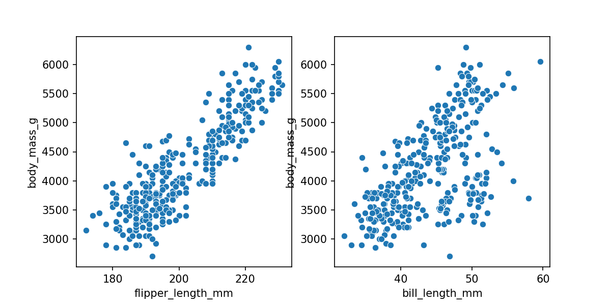
From the previous module we already knew there was a clear linear relationship between flipper length and body mass. There is also the same general relationship of increasing mass with increasing bill length. We'll use this additional feature/parameter to predict the body mass.

Follow Along

We'll follow the same steps to fit the model, except our feature matrix will have an additional dimension.

# Remove NaN before creating features
penguins.dropna(inplace=True)

# Create the 2-D features matrix
features = ['flipper_length_mm', 'bill_length_mm']
X_penguins = penguins[features]

# Create the target vector
y_penguins = penguins['body_mass_g']

# Import the estimator class
from sklearn.linear_model import LinearRegression

# Instantiate the class (with default parameters)
model = LinearRegression()

# Fit the model
model.fit(X_penguins, y_penguins)

LinearRegression()

# Slope (2 parameters here)
print(model.coef_)

# Intercept
print(model.intercept_)

[48.88969177  4.95860126]
-5836.298732120461

As we expected, the model fit returns two regression coefficients. If we go back to the equations for a multiple linear regression and substitute in our coefficients, we now have the equation of a plane instead of a line:

$y = -5836 + 49X_{1} + 5X_{2}$

Both of the regression coefficients are positive, which means that as the flipper length and bill length increase, the mass of the penguin also increases.

Since we have two features, we need an additional dimension on our plot. We could do this with color shading or even try to create a 3D plot. We'll put our data in a format that's easier to plot.

# Format the data for plotting
x_flipper = penguins['flipper_length_mm']
y_bill = penguins['bill_length_mm']
z_weight = penguins['body_mass_g']

# Create the data to plot the best-fit plane
(x_plane, y_plane) = np.meshgrid(np.arange(165, 235, 1), np.arange(30, 60, 1))
z_plane = -5836 + 49*x_plane + 5*y_plane

# Import for plotting
import matplotlib.pyplot as plt
from mpl_toolkits.mplot3d import Axes3D
from matplotlib import cm

# Initial the figure and axes objects
fig = plt.figure(figsize=(6,6))
ax = fig.add_subplot(111, projection='3d')

# Plot the data: 2 features, 1 target
ax.scatter(xs=x_flipper, ys=y_bill, zs=z_weight, zdir='z', 
           s=20, c=z_weight, cmap=cm.viridis)

# Plot the best-fit plane
ax.plot_surface(x_plane, y_plane, z_plane, color='gray', alpha = 0.5)

# General figure/axes properties
ax.view_init(elev=28, azim=325)
ax.set_xlabel('Flipper length')
ax.set_ylabel('Bill length')
ax.set_zlabel('Body mass')
fig.tight_layout()

plt.show()
plt.clf()

mod2_obj2_multireg_3D

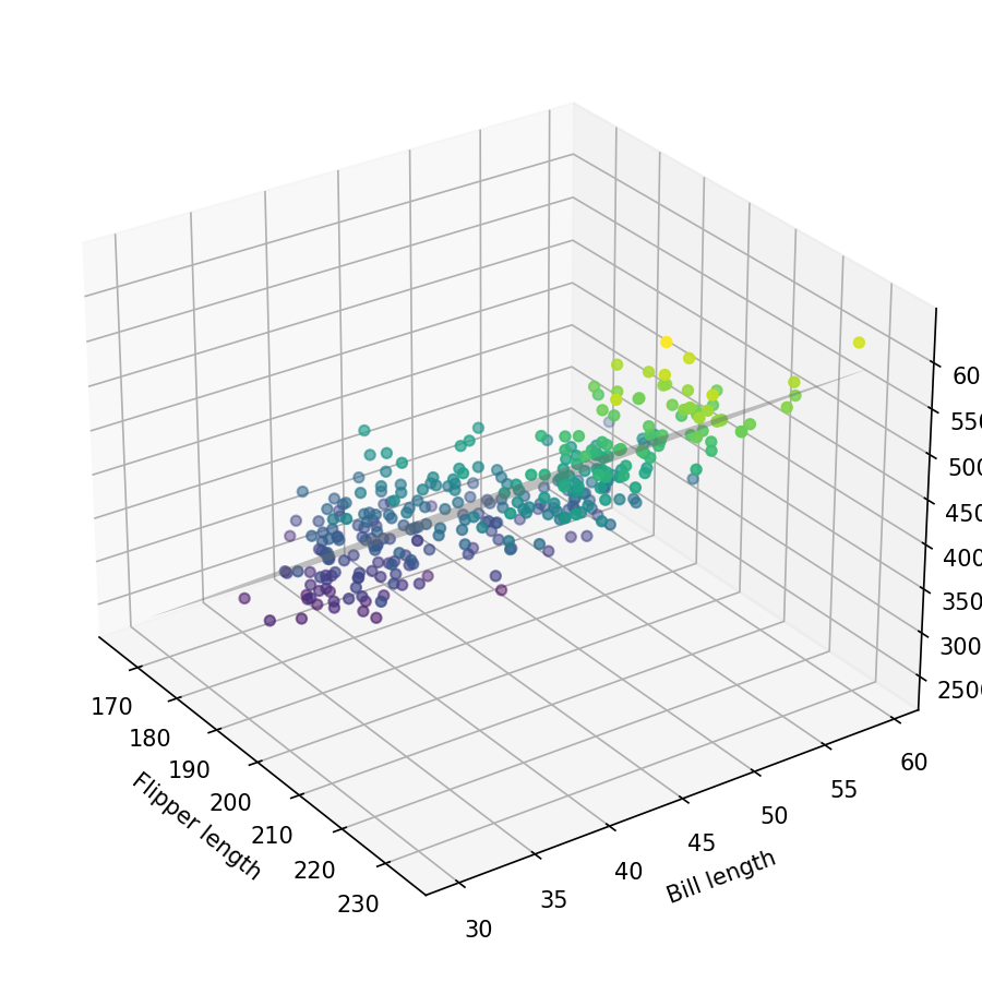
In the above plot, we have our penguin data (colored circles) and the best-fit plane (gray). Since this is a static plot it's difficult to view the distribution of data from other angles. But we can see that with increasing flipper and bill lengths, the mass also increases.

Challenge

Now it's your turn! There is one additional feature in the penguins data set that we didn't plot (the bill width or "beak" width). Using the same code as above, substitute in the variable "bill_width_mm" for the "bill_length_mm". Does this feature show a linear relationship with body mass?

Additional Resources

Objective 03 - Understand how ordinary least squares regression minimizes the sum of squared errors

Overview

So far, we have fit a simple linear regression with one feature and a multiple linear regression with two features. These two processes were relatively easy to do because we used the scikit-learn predictor to fit models to our data.

How do these estimators actually determine the parameters (regression coefficients) for our models? The answer includes a lot of math! In this objective we'll take a closer look at the mathematics behind an ordinary least squares (OLS) regression and how it works.

Sum of squared errors

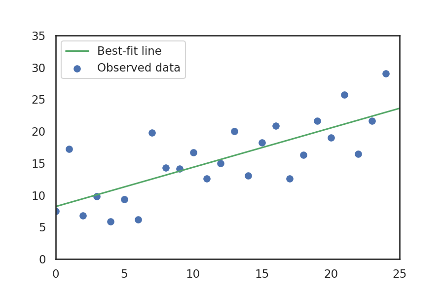
The ordinary least squares method is based on minimizing the sum of the squared error. This error is the difference between the observed dependent variable and the value predicted by the linear model. The OLS method estimates the slope and intercept parameters for a line, that minimizes the sum of the squared distances between the line and the observed data.

OLS plot

Math: sum of squares

Looking at the plot above we can see that each data point is some distance away from the line, as measured along the y axis. To determine how well a given line fits the observed data, we sum the square of the distance of each point from the line. Some of the data is above the line (positive distance) and some is below (negative distance). We square this distance so that the negative values don't cancel out the positive values.

The form of the equation for a line takes many forms and uses different variables. We've been using $y = \beta_0 + \beta_1X_1$ and we'll continue with this format. It is important to be aware that there are other variables used for the parameters in the equation of a line. We'll start with an equation for a line with the form:

$y = \beta_0 + \beta_1X$

We want to estimate the parameters for $\beta_0$ and $\beta_1X$ . For each data point in our data set, we want to find the value predicted by using the coefficients $\beta_0$ and $\beta_1$ . The predicted value of y would be given by:

$y_{predict} = \beta_0 + \beta_1x_i$

The error or residual between the actual value y_i and the predicted value $y_{predict}$ is:

$\text{diff} = y_{i} - y_{predict} = y_{i} - (\beta_0 + \beta_1x_{i})$

We want to sum over all of the error values in the data set. So we need to square this difference and then add them up:

$\text{Sum of squares} = \sum (y_{i} - (\beta_0 + \beta_1 x_{i}))^2$

Now comes the fun part: we need to apply some math to the above sum of squares equation to find the values of and that minimize the sum. There are a few different ways to derive this answer, including using calculus and linear algebra. These derivations are beyond the scope of this course, so we're going to go straight to the answer.

Parameter estimates: least squares

The values for the parameters are given by:

$\beta_1 = \frac{Cov[x,y]}{Var[x]}$

$\beta_0 = \bar{y} - \beta_1 \bar{x}$

where $\bar{x}$ and $\bar{y}$ are the mean values of and .

Follow Along

Now that we have some of the math out of the way, let's code a simple example to find the coefficients for a linear regression. Instead of using a real-world data set, it will be easier to generate a small sample data set where we determine the coefficients.

# Import numpy
import numpy as np

# Generate the sample data
x = np.arange(25)
delta = np.random.uniform(0,20, size=(25,))
y = 0.4 * x + 3 + delta

# Define a function to calculate alpha and beta

def least_squares_params(x, y):
    '''
    x and y: data to be fit
    returns: the least-square values of alpha and beta
    '''
    # Calculate the mean of X and y
    xmean = np.mean(x); ymean = np.mean(y)

    # Calculate the covariance for x and y, variance for x
    xycov = (x-xmean)*(y-ymean)
    xvar = (x-xmean)**2

    # Calculate the coefficients
    beta_1 = sum(xycov) / sum(xvar)
    beta_0 = ymean - (beta_1*xmean)

    print('beta_0: ', beta_0)
    print('beta_1: ', beta_1)

Now that we have a reasonably simple function, let's try it out on the data we generated above.

# Find the estimated parameters for alpha, beta
# given our (x, y) data set
least_squares_params(x,y)

beta_0:  11.01787535843764
beta_1:  0.5507176494641995

We estimated the parameters! How do we know that they are correct? It's possible there could be an error in our function or that we didn't use the correct formula for estimating the parameters.

A quick check would be to use the scikit-learn estimator and find the coefficients. We've already done this a few times, but let's do it one more time for practice.

# Import the estimator class
from sklearn.linear_model import LinearRegression

# Instantiate the class (with default parameters)
model = LinearRegression()

X = x[:, np.newaxis]

# Fit the model
model.fit(X, y)

# Intercept
print('beta_0: ', model.intercept_)

# Slope (also called the model coefficient)
print('beta_1: ', model.coef_)

beta_0:  11.017875358437646
beta_1:  [0.55071765]

It looks like our estimator function above was correct. The results from the scikit-learn LinearRegression model are the same.

Challenge

This objective covered a lot of material. The best way to continue to practice would be to try it for yourself. Following the example above, use a different data set and calculate the coefficients using the function provided above. Then, fit a scikit-learn regression model to the data and confirm that it calculates the same model coefficients as our custom approach.

Additional Resources

Khan Academy: Squared Error of Regression

Objective 04 - Define overfitting-underfitting and the bias-variance tradeoff

Overview

Earlier in this module, we introduced how to separate our data into training and testing sets. The main reason to do this is to verify the results of our model on new data or data the model hasn't yet seen. The more formal term is overfitting or producing a model that performs well on our training data but doesn't generalize well to our test data (or other new data).

The opposite problem also occurs, where we can underfit a model meaning it doesn't do well even on the training data. In this case, you would probably need to choose a different model to fit. In general, underfitting is not as common as overfitting.

Follow Along

Example: overfitting vs. underfitting

To better understand model fitting, let's use an example where we have fit a polynomial (curve) to a small data set. There are three polynomials fit to the data: a first degree (which is just a line), a sixth degree, and a ninth degree. The degree of a polynomial indicates how many nonzero coefficients it has. The higher the degree, the more parameters can be fit to the data.

over-under

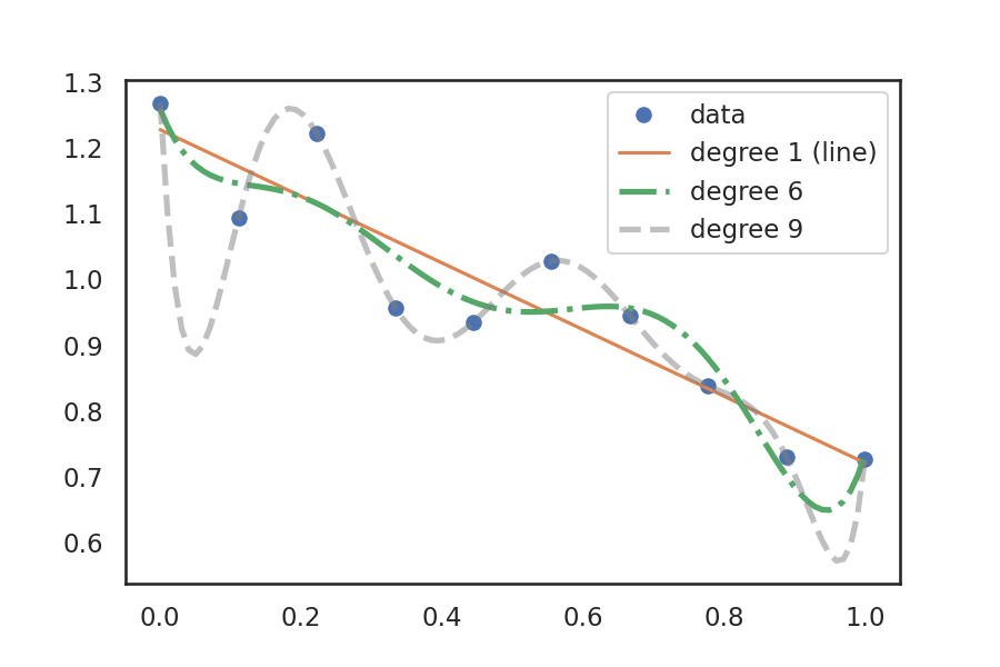
The line already fits the data reasonably well, but is still probably underfit. The sixth degree polynomial is an example of overfitting, where the model will probably not fit new data very well. The ninth degree polynomial nicely goes through every data point but needs to make several dips to fit. This model would provide a very poor result when used on new unseen data.

Bias and variance

The concepts of underfitting and overfitting are also related to bias and variance. A high bias model makes a lot of mistakes in fitting the model. The first degree polynomial model is an example. But, if we fit this 1-degree model to a different training set, it will likely have similar results. This type of model has a high bias and low variance.

On the other end, the 9-degree model fits the data almost perfectly. But, if we trained the model on a different training set, the results would be very different. The curve would not look the same. This type of model has low bias but a high variance.

High bias: Doesn't pay a lot of attention to the data and over simplifies the model
Low bias: Pays too much attention to the data and is usually a complicated model
High variance: Fits the training data set very well but doesn't generalize to new data
Low variance: Returns similar models for different sets of training data

Additional Resources

Ask a Data Scientist: The Bias vs. Variance Tradeoff

Guided Project

Open JDS_SHR_212_guided_project_notes.ipynb in the GitHub repository below to follow along with the guided project:

GitHub: Linear Regression II Slides

Guided Project Video

Module Assignment

Complete the Module 2 assignment to practice advanced linear regression techniques you've learned.

Module 2: Linear Regression 2

Module Overview

Learning Objectives

Objective 01 - Implement a train-test split with scikit-learn

Overview

Train-test Split

Scikit-learn Train-test

Follow Along

Create Training and Test Sets

Making predictions

Additional Resources

Objective 02 - Use scikit-learn to fit a multiple regression

Overview

Multiple Linear Regression

Follow Along

Challenge

Additional Resources

Objective 03 - Understand how ordinary least squares regression minimizes the sum of squared errors

Overview

Sum of squared errors

Math: sum of squares

Parameter estimates: least squares

Follow Along

Challenge

Additional Resources

Objective 04 - Define overfitting-underfitting and the bias-variance tradeoff

Overview

Follow Along

Example: overfitting vs. underfitting

Bias and variance

Additional Resources

Guided Project

Guided Project Video

Module Assignment

Assignment Solution Video

Resources

Datasets

Documentation and Tutorials

Articles and Readings