DS3 Module 3 - Linear Algebra

Module Overview

In this module, you will learn about the fundamentals of linear algebra and its applications in data science. You'll explore vectors, matrices, linear transformations, and how they relate to linear regression models. These concepts form the mathematical foundation for many machine learning algorithms.

Learning Objectives

Define a Vector and Calculate a Vector Length and Dot Product
Explain Cosine Similarity and Compute the Similarity Between Two Vectors
Define a Matrix and Calculate a Matrix Dot Product, Transpose, and Inverse
Use Linear Algebra to Solve for Linear Regression Coefficients

Objective 01 - Define a Vector and Calculate a Vector Length and Dot Product

Overview

We're finally getting to the topic you have been waiting for: linear algebra. This module aims not to teach you a lot of linear algebra but instead to introduce you to the basics to begin to apply those concepts to your work.

Follow Along

We're going to introduce the notation used in linear algebra and repeat the Python calculations so that you will have practice with both. You do not need to work through the material in this section by hand, but please do so if that helps you better understand the concepts!

Vectors

You may have already encountered vectors in a science or math class: a vector has magnitude and direction. That type of vector was probably a two-dimensional vector that was easy to graph on paper and then measure its properties. As we'll see later in this section, it's relatively easy to plot two- and three-dimensional vectors. But first, let's look at the notation and create some vectors.

Two-dimensional vector:

$\vec{a} = \begin{bmatrix}7 & 9\end{bmatrix}$

Three-dimensional vector:

$\vec{b} = \begin{bmatrix}4 & 7 & 2\end{bmatrix}$

A characteristic of a vector is its dimension. Of course, a vector can have infinite dimensions, but we're going to stick to vectors with much lower dimensions. Here's an example of an 11-dimension vector:

$\vec{c}=[3 \space1\space 4\space1\space 5\space 9\space 2\space 6\space 5\space 3\space 5]$

Let's rewrite our vectors, but this time we'll express them in Python. The numpy library you have already been using has a data structure called an array, which is essentially a vector.

import numpy as np

# Two-dimensonal vector
my_2dvector = np.array([7, 9])
print('2D vector:', my_2dvector)

# Three-dimensonal vector
my_3dvector = np.array([4, 7, 2])
print('3D vector:', my_3dvector)

2D vector: [7 9]
3D vector: [4 7 2]

We can also plot the two- and three-dimensional vectors. Unfortunately, because we live in a three-dimensional world, we can't easily visualize the dimensions beyond that. But that doesn't mean the higher dimensional vectors aren't helpful - they are, and we'll be using them throughout the course.

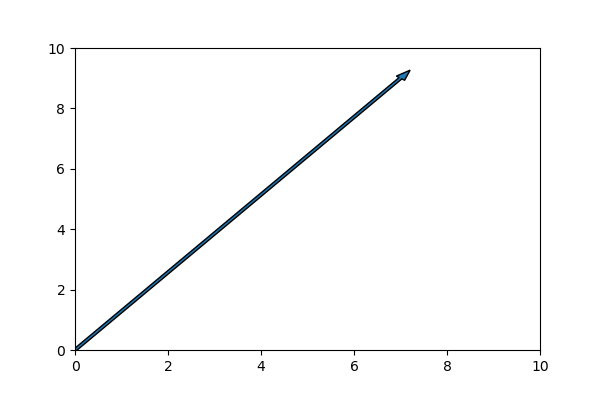
First, we'll plot our two-dimensional vector :

$\vec{a} = \begin{bmatrix}7 & 9\end{bmatrix}$

Think of it as extending seven units in the x-direction and none-units in the y-direction.

import matplotlib.pyplot as plt
%matplotlib inline

fig, ax = plt.subplots(1,1)
ax.arrow(0, 0, 7, 9, width=.075)
ax.set_xlim([0, 10]); ax.set_ylim([0, 10])

#plt.show()

plt.clf()

<Figure size 432x288 with 0 Axes>
mod4_obj1_vector1.png

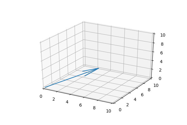
Then we'll plot our three-dimensional vector. Again, think of it as extending four units in the x-direction, seven units in the y-direction, and two units in the z-direction.

from mpl_toolkits import mplot3d

# 3D vector
c = [4,7,2]
vector = np.array([[0, 0, 0, c[0], c[1], c[2]]])
# Create variables for plotting
X, Y, Z, U, V, W = zip(*vector)
# Plot!
ax = plt.axes(projection='3d')
ax.quiver(X, Y, Z, U, V, W, length=1)
ax.set_xlim([0, 10]); ax.set_ylim([0, 10]); ax.set_zlim([0, 10])

plt.clf()

<Figure size 432x288 with 0 Axes>

Plotting a 2D vector was pretty easy; plotting the 3D vector begins to involve more code. But it's important to visualize even these simple vectors.

Row and Column vectors

Vectors are defined as a row vector:

$\vec{a} = \begin{bmatrix}8 & 6 & 7 & 5 & 3 & 0 & 9\end{bmatrix}$

And they can be defined as a column vector:

$\vec{a} = \begin{bmatrix}8 \\ 6 \\ 7 \\ 5 \\ 3 \\ 0 \\ 9\end{bmatrix}$

Now we'll look at these same vectors expressed as numpy arrays in Python.

# Row vector
my_row_vector = np.array([8,6,7,5,3,0,9])
print('Row vector:', my_row_vector)

# Column vector
# reshape(-1,1): specifies one column, unknown rows 
my_column_vector = np.array([8,6,7,5,3,0,9]).reshape(-1,1)
print('Column vector:\n', my_column_vector)

Row vector: [8 6 7 5 3 0 9]
Column vector:
 [[8]
 [6]
 [7]
 [5]
 [3]
 [0]
 [9]]

Vector Math

Vector length

We can also do math with vectors. As we said earlier, vectors have a magnitude and direction. The magnitude of a vectors is just it's length. We determine the length by taking the sum of the squares of each element and then take the square root:

Three-dimensional vector:

$\vec{b} = \begin{bmatrix}4 & 7 & 2\end{bmatrix}$

$||\vec{b}|| = \sqrt{b_1^2 + b_2^2 + b_3^2} = \sqrt{4^2 + 7^2 + 2^2} = \sqrt{16+49+4} = \sqrt{69} = 8.3$

Vector dot product

The dot product is a kind of multiplication where we're applying one vector to another. It can also be thought of as applying the directional growth of one vector to another.

We'll calculate the dot product for vectors $\vec{b}$ and $\vec{ c}$ :

$\vec{b} = \begin{bmatrix}4 & 7 & 2\end{bmatrix} \qquad \vec{c} = \begin{bmatrix} 6 & 1 & 7\end{bmatrix}$

The dot product notation looks like this:

$\vec{b} \cdot \vec{c}$

It represents the sum of the element-wise multiplication of the two vectors:

$\vec{b} \cdot \vec{c} = b_{1}c_{1} + b_{2}c_{2} + b_{3}c_{3}$ = (4)(6) + (7)(1) + (2)(7) = 24 + 7 + 14 = 45

We can also do vector math in Python. Let's reproduce the vector length and dot product calculations we just did, only using numpy.

# Vector length
b = np.array([4, 7, 2])
np.linalg.norm(b)

8.306623862918075

# Dot product of two arrays (vectors)
b = np.array([4, 7, 2])
c = np.array([6, 1, 7])
np.dot(b, c)

Both of our calculations agree!

Challenge

Now it's your turn. Here are a few tasks to practice:

plot a vector (make sure to change the limits on your plot if needed)
create and print out both row and column vectors (in Python)
calculate the length of your vector (in Python)
take the dot product of two vectors (in Python)

Additional Resources

Objective 02 - Explain Cosine Similarity and Compute the Similarity Between Two Vectors

Overview

Now that we've had some practice with vectors and a few associated math operations, we can start learning about more exciting concepts. In some situations, we may want to know more than the length of a vector or its dot product with another vector. For example, comparing the similarity of vectors is vital in natural language processing, where a vector can represent words themselves.

To compare the similarity of two vectors, we need to determine something called the cosine similarity.

Cosine similarity

We use cosine similarity when we want to compare vectors and how similar they are. The angle between vectors is a measure of their similarity. First, let's look at vectors that point in the same direction and those in the opposite direction.

# Import libraries
import numpy as np
import matplotlib.pyplot as plt
%matplotlib inline

# Plot identical and opposite vectors

fig, [ax1, ax2, ax3] = plt.subplots(1,3, figsize=(12,3))

# vector1 = [2, 4]; vector2 = [4, 8]
# Same direction, y is twice as long
ax1.arrow(0, 0, 2, 4, color='k', width=.15)
ax1.arrow(0, 0, 4, 8, color='orange', width=.075)
ax1.set_xlim([-1, 10]); ax1.set_ylim([-1, 10])
ax1.set_title("Vectors: same direction")

# vector1 = [0, 4]; vector2 = [4, 0]
# Right angle vectors
ax2.arrow(0, 0, 0, 4, color='k', width=.075)
ax2.arrow(0, 0, 4, 0, color='orange', width=.075)
ax2.set_xlim([-1, 10]); ax2.set_ylim([-1, 10])
ax2.set_title("Vectors: perpendicular")

# vector1 = [-2, -2]; vector2 = [2, 2]
# Same length, opposite direction
ax3.arrow(4, 4, -2, -2, color='k', width=.075)
ax3.arrow(4, 4, 2, 2, color='orange', width=.075)
ax3.set_xlim([-1, 10]); ax3.set_ylim([-1, 10])
ax3.set_title("Vectors: opposite direction")

plt.savefig('/Users/nicole/data_science_LS/data-science-canvas-images/unit_1/sprint_3/new/mod4_obj2_vector_angles.png',
           transparent=False, dpi=100)

#plt.show()
plt.clf()

<Figure size 864x216 with 0 Axes>

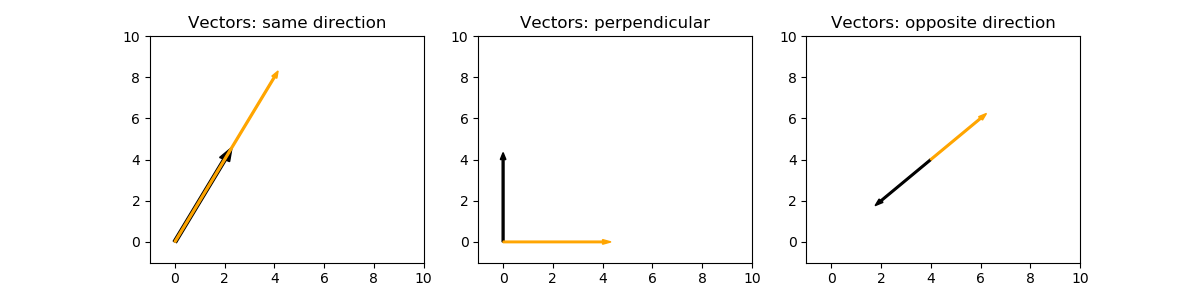
On the plot on the left, the vectors point in the same direction. The orange (lighter colored) vector is twice as long as the black vector. The angle between the vectors is 0. On the right, the vectors have the same length but point in the opposite direction. The angle between them is 180 degrees. The middle plot has perpendicular (or orthogonal) vectors to each other, and the angle between them is 90 degrees.

Remember that the cosine is the angle between the hypotenuse and the adjacent side of a triangle.

cosine

The cosine of the angle is written as the length of the adjacent side over the length of the hypotenuse:

$\cos \theta = \frac{adjacent}{hypotenuse}$

Cosine function for different values of $\theta$:

$\cos 0 = 1$
$\cos 90 = 0$
$\cos 180 = -1$

Let's plot a pair of vectors where the angle between them is not 0, 90, or 180 degrees:

# Vector plots

x = np.array([6, 4])
y = np.array([3, 7])

fig, ax = plt.subplots(1,1)
ax.arrow(0, 0, x[0], x[1], color='k', width=.075)
ax.arrow(0, 0, y[0], y[1], color='orange', width=.075)
ax.set_xlim([-1, 10]); ax.set_ylim([-1, 10])

plt.show()
plt.clf()

<Figure size 432x288 with 0 Axes>

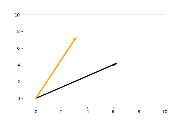
These vectors point in different directions. We can calculate the cosine of the angle between these vectors (or any two vectors) with the following equation:

For vectors $\mathbf {A}$ and $\mathbf {B}$ :

$\mathbf {A} \cdot \mathbf {B} =\left\|\mathbf {A} \right\|\left\|\mathbf {B} \right\|\cos \theta$

Solving for $\cos \theta$ we get

$\cos \theta= \frac{\mathbf {A} \cdot \mathbf {B} }{\left\|\mathbf {A} \right\|\left\|\mathbf {B} \right\|}$

The quantity $\mathbf {A} \cdot \mathbf {B}$ is the dot product and $\left\|\mathbf {A} \right\|\left\|\mathbf {B} \right\|$ is the product of the lengths of the vectors.

Let's use Python to calculate the cosine of the angle between these vectors.

# Calculate cosine theta

# Vectors
x = np.array([6, 4])
y = np.array([3, 7])

# Cosine theta (cosine similarity)
np.dot(x, y) / (np.linalg.norm(x) * np.linalg.norm(y))

0.8376105968386142

Our value for $\cos \theta = 0.84$ is between -1 and 1 as we expected. If the vectors had an angle of 0, we’d have a result of 1; since these vectors have an angle a little bit more than 0 degrees, the value for $\cos \theta$ is slightly smaller than 1.

Challenge

Try doing your own $\cos \theta$ calculations. You should try to plot the vectors first and then calculate the cosine similarity and see if it agrees with what you think it should be.

Additional Resources

Objective 03 - Define a Matrix and Calculate a Matrix Dot Product, Transpose, and Inverse

Overview

Now that we've practiced some mathematical operations with vectors, we can continue to expand our linear algebra knowledge and move onto matrices. As with vectors, you've probably also worked with matrices in Python without really focusing on what they were.

Remember the column vector from earlier in the module? We can think of a column vector as a one-dimensional matrix. If we add more columns, then we have additional dimensions and a matrix.

Column vector: $\vec{a} = \begin{bmatrix}1 \\ 4 \\ 7 \end{bmatrix}$

Let's combine some more column vectors (not addition but just adding more columns):

$\text{Combining this vector}\begin{bmatrix}1 \\ 4 \\ 7 \end{bmatrix} \text{and this one} \begin{bmatrix}2 \\ 5 \\ 8 \end{bmatrix} \text{results in this matrix}$

$M = \begin{bmatrix} 1 & 2 \\ 4 & 5 \\ 7 & 8 \end{bmatrix}$

Matrices are represented with an upper case letter:

$M = \begin{bmatrix} 1 & 2 & 3 \\ 4 & 5 & 6 \\ 7 & 8 & 9 \end{bmatrix}$

We create matrices in Python using numpy and adding additional column dimensions. Recall that the dimension of a vector is just its length. So we'll have a matrix if we add additional rows to a row vector or additional columns to a column vector. Because we have both, number of rows and a number of columns, we need to talk about the matrix as 'n' rows by 'm' columns; a 2x2 matrix would have two rows and two columns.

Let's create some matrices of different dimensions.

import numpy as np

# Two dimensional numpy array (2x3)
matrix1 = np.array([[ 1, 2, 3],[ 4, 5, 6]])
print('2x3 matrix:\n', matrix1)

# 3x3 numpy array
matrix2 = np.array([[ 1, 2, 3],[ 4, 5, 6], [7, 8, 9]])
print('\n3x3 matrix:\n', matrix2)

2x3 matrix:
 [[1 2 3]
 [4 5 6]]

3x3 matrix:
 [[1 2 3]
 [4 5 6]
 [7 8 9]]

Matrix Math

We'll go over a few basic matrix operations. Of course, there are many more, but there are several excellent resources available for further review.

Matrix multiplication

We accomplish matrix multiplication by calculating the dot product between the rows of the first matrix and the columns of the second matrix. This image from Math is Fun is a good illustration.

Let's multiply two matrices and then check the results with Python.

$X = \begin{bmatrix} 1 & 4 & 8 \\ 2 & 3 & 1 \\ \end{bmatrix}$

$Y = \begin{bmatrix} 1 & 6 \\ 2 & 3 \\ 5 & 7 \end{bmatrix}$

$X Y = \begin{bmatrix} (1)(1)+(4)(2)+(8)(5) & (1)(6)+(4)(3)+(8)(7) \\ (2)(1)+(3)(2)+(1)(5) & (2)(6)+(3)(3)+(1)(7) \end{bmatrix}$

$X Y = \begin{bmatrix} 49 & 74 \\ 13 & 28 \end{bmatrix}$

# Check matrix multiplication with Python

X = np.array([[1,4,8],[2,3,1]])
Y = np.array([[1,6],[2,3],[5,7]])

X_Y = np.matmul(X, Y)
print('X * Y:\n', X_Y)

X * Y:
 [[49 74]
 [13 28]]

Matrix Transpose

The transpose of a matrix is essentially swapping the rows and columns.

Wikipedia Matrix Transpose

We write the transpose with a superscript T: M^T .

We can easily take the transpose of a matrix in numpy.

A = np.array([[1, 2], [3, 4],[5, 6]])
print('Original matrix:\n', A)

A_T = np.transpose(A)
print('Transposed matrix:\n', A_T)

Original matrix:
 [[1 2]
 [3 4]
 [5 6]]
Transposed matrix:
 [[1 3 5]
 [2 4 6]]

Inverse of a Matrix

In the same way that a number can have a reciprocal, where

4 has the inverse 1/4.

a matrix can have an inverse, where

A has the inverse A^{-1}.

You use a superscript because you cannot divide by a matrix.

Identity Matrix

The identity matrix is a specific diagonal matrix where there are only ones on the main diagonal and zeros everywhere else. This matrix acts a lot like the number 1: if we multiply any matrix by its identity matrix, the original matrix will remain unchanged. Here's an example of a 3x3 identity matrix.

$I_3 = \begin{bmatrix} 1 & 0 & 0 \\ 0 & 1 & 0 \\ 0 & 0 & 1 \end{bmatrix}$

Challenge

For this challenge, practice creating some matrices in Python (numpy arrays) and then calculate the:

matrix multiplication
multiplying by the identity matrix
calculating the transpose

Additional Resources

Objective 04 - Use Linear Algebra to Solve for Linear Regression Coefficients

Overview

The material in this sprint has been a combination of exploring linear regression and making inferential statements. And we've also introduced some linear algebra basics. Now we will combine the two and look at how to state a linear regression model with vectors and matrices.

Linear Regression

Recall the form of the linear regression equation (for one independent variable):

y = b_0 + b_1x

Now we're going to consider each individual data point we have in our data set - we'll start with the first, then second, etc.:

y_1 = b_0 + b_1x_1

y_2 = b_0 + b_1x_2

y_3 = b_0 + b_1x_3

we can generalize by using i for each data point:

y_i = b_0 + b_1x_i

Let's write our target (dependent) variables as a vector and our independent variable also as a vector.

$\begin{bmatrix} y_1 \\ y_2 \\ y_3 \\ \vdots \\ y_i \end{bmatrix} = \begin{bmatrix} b_0 \\ b_0 \\ b_0 \\ \vdots \\ b_0 \end{bmatrix} + \begin{bmatrix} b_1x_1 \\ b_1x_2 \\ b_1x_3 \\ \vdots \\ b_1x_i \end{bmatrix}$

We can further simplify this equation by pulling the b coefficients out of the matrix, and writing them in their own vector:

$\begin{bmatrix} b_0 \\ b_1 \end{bmatrix}$

The equation now has this form:

$\begin{bmatrix}y_1 \\ y_2 \\ y_3 \\ \vdots \\ y_i \end{bmatrix} = \begin{bmatrix}1 & x_1 \\ 1 & x_2 \\ 1 & x_3 \\ \vdots \\ 1 & x_i \end{bmatrix} \begin{bmatrix}b_0 \\ b_1 \end{bmatrix}$

We can write this in matrix form as:

Y = BX

Solve for the linear regression coefficient

Now, let's put to use what we've learned working with matrices and solve for B. Okay, this involves quite a lot of linear algebra and some calculus. What we want is the least-squares solution to the above equation. Remember the ordinal least-square (OLS) model we used in the previous modules? The least-squares solution is:

$B = (X^T X)^{-1}X^TY$

where X^T is the transpose of X.

Now let's load in the car crash data set, create the X matrix and Y vector and solve for the coefficients for the linear regression.

Follow Along

First, we need the data. Recall that we are looking at the relationship between alcohol impairment (alcohol) and the total number of accidents (total).

import pandas as pd
import seaborn as sns

# Load the car crash dataset
crashes = sns.load_dataset(" car_crashes") crashes.head()

	total	speeding	alcohol	not_distracted	no_previous	ins_premium	ins_losses	abbrev
0	18.8	7.332	5.640	18.048	15.040	784.55	145.08	AL
1	18.1	7.421	4.525	16.290	17.014	1053.48	133.93	AK
2	18.6	6.510	5.208	15.624	17.856	899.47	110.35	AZ
3	22.4	4.032	5.824	21.056	21.280	827.34	142.39	AR
4	12.0	4.200	3.360	10.920	10.680	878.41	165.63	CA

Now, we'll put the data into the appropriately shaped vector and matrix. We have two columns in the X matrix: a column of ones and a column with the data points for the alcohol feature.

# Create independent (feature) matrix
import numpy as np

# Create the ones column
ones = np.repeat(1,len(crashes)).reshape(-1,1)

# Select a column and reshape to add an additional column
alcohol = np.array(crashes['alcohol']).reshape(-1,1)

# "Glue" the columns together
X = np.concatenate((ones, alcohol), axis=1)

# Look at the shape
print('The feature matrix has a shape:', X.shape)

# Create the dependent (target) vector
Y = np.array(crashes['total']).reshape(-1,1)

print('The target vector has a shape:', Y.shape)

The feature matrix has a shape: (51, 2)
The target vector has a shape: (51, 1)

Now we can make Python do all of the linear algebra for us!

# Calculate X transpose
X_T = np.transpose(X)

# Calculate X transpose multiplied by X
X_T_X = np.matmul(X_T,X)

print('X transpose multiplied by X:\n', X_T_X)

# Calculate the inverse of X_T_X
X_T_X_inv = np.linalg.inv(X_T_X)

print('\nInverse of X transpose multiplied by X):\n', X_T_X_inv)

#Calculate X transpose Y
X_T_Y = np.matmul(X_T,Y)

print('\nX transpose multiplied by Y:\n', X_T_Y)

# Finally - calculate B =  = (X'X)^-1 multiplied by X'Y

B = np.matmul(X_T_X_inv,X_T_Y)

print('\nThe regression coefficients B are:\n', B)

X transpose multiplied by X:
 [[  51.        249.226   ]
 [ 249.226    1367.408738]]

Inverse of X transpose multiplied by X):
 [[ 0.17935002 -0.03268861]
 [-0.03268861  0.00668919]]

X transpose multiplied by Y:
 [[ 805.3  ]
 [4239.177]]

The regression coefficients B are:
 [[5.85777615]
 [2.0325063 ]]

Let's compare these coefficients to the ones we find using the scikit-learn LinearRegression() model.

# Import the predictor class
from sklearn.linear_model import LinearRegression

# Instantiate the class (with default parameters)
model = LinearRegression()

# Change the format slightly of X (we just need one column, no ones)
X = np.array(crashes['alcohol']).reshape(-1,1)

# Fit the model
model.fit(X, Y)

# Intercept (b_0)
print('The intercept(b_0): ', model.intercept_)

# Slope (b_1)
print('The slope (b_1):', model.coef_)

The intercept(b_0):  [5.85777615]
The slope (b_1): [[2.0325063]]

Well look at that - the result of doing the calculation "by hand" (writing out the linear algebra) agrees with the scikit-learn regression model. But since the computer uses linear algebra "under the hood", we would hope everything agrees.

Challenge

Since we covered a lot of content in this objective, the best thing to do is review the above. First, go over the steps to write the linear regression equation in matrix form and make sense. Then, look through the code for how B was determined (you don't need to look up the derivation, but some resources at the end provide further information).

Additional Resources

Guided Project

Open DS_133_Linear_Algebra.ipynb in the GitHub repository below to follow along with the guided project:

GitHub: Linear Algebra

Guided Project Video

Module Assignment

Complete the Module 3 assignment to practice linear algebra techniques you've learned.

Module 3: Linear Algebra

Module Overview

Learning Objectives

Objective 01 - Define a Vector and Calculate a Vector Length and Dot Product

Overview

Follow Along

Vectors

Row and Column vectors

Vector Math

Vector length

Vector dot product

Challenge

Additional Resources

Objective 02 - Explain Cosine Similarity and Compute the Similarity Between Two Vectors

Overview

Cosine similarity

cosine

Challenge

Additional Resources

Objective 03 - Define a Matrix and Calculate a Matrix Dot Product, Transpose, and Inverse

Overview

Matrix Math

Matrix multiplication

Matrix Transpose

Inverse of a Matrix

Identity Matrix

Challenge

Additional Resources

Objective 04 - Use Linear Algebra to Solve for Linear Regression Coefficients

Overview

Linear Regression

Solve for the linear regression coefficient

Follow Along

Challenge

Additional Resources

Guided Project

Guided Project Video

Module Assignment

Assignment Solution Video

Resources

Documentation and Tutorials

Videos