Module 2: Multiple Regression
Module Overview
In this module, you will learn about multiple regression. You'll explore how to model relationships with multiple predictor variables, conduct t-tests to determine variable significance, and compare model fit using adjusted R-squared.
Learning Objectives
- Model the Relationship of Multiple Predictor Variables to a Single Outcome
- Conduct a t-test to Determine the Significance of Individual Variables in the Model
- Compare Model Fit Using Adjusted R-squared
Objective 01 - Model the Relationship of Multiple Predictor Variables to a Single Outcome
Overview
The previous module fit a linear regression model to two variables in our car crash data set: total accidents and alcohol impairment. We found a significant relationship between the two variables and could reject the null hypothesis.
In this module, we will look at how adding multiple predictor variables to a linear regression affects the outcome. Can we improve the linear regression model by adding in more predictor variables? First, let's load in the data, fit the model, and look at the results.
Follow Along
For this module, we'll look at the whole data set again, instead of just focusing on two variables.
import seaborn as sns

# Load the car crash dataset
crashes = sns.load_dataset("car_crashes")

crashes.head()| total | speeding | alcohol | not_distracted | no_previous | ins_premium | ins_losses | abbrev | |
|---|---|---|---|---|---|---|---|---|
| 0 | 18.8 | 7.332 | 5.640 | 18.048 | 15.040 | 784.55 | 145.08 | AL |
| 1 | 18.1 | 7.421 | 4.525 | 16.290 | 17.014 | 1053.48 | 133.93 | AK |
| 2 | 18.6 | 6.510 | 5.208 | 15.624 | 17.856 | 899.47 | 110.35 | AZ |
| 3 | 22.4 | 4.032 | 5.824 | 21.056 | 21.280 | 827.34 | 142.39 | AR |
| 4 | 12.0 | 4.200 | 3.360 | 10.920 | 10.680 | 878.41 | 165.63 | CA |
We'll fit our model using alcohol as the independent variable and total as the
dependent variable.
import seaborn as sns
from statsmodels.formula.api import ols

crashes = sns.load_dataset("car_crashes")

# Set-up and fit the model in one step
model = ols("total ~ alcohol", data=crashes).fit()

print(model.summary())
                            OLS Regression Results
==============================================================================
Dep. Variable:                  total   R-squared:                       0.727
Model:                            OLS   Adj. R-squared:                  0.721
Method:                 Least Squares   F-statistic:                     130.5
Date:                Wed, 21 Apr 2021   Prob (F-statistic):           2.04e-15
Time:                        13:48:00   Log-Likelihood:                -110.99
No. Observations:                  51   AIC:                             226.0
Df Residuals:                      49   BIC:                             229.8
Df Model:                           1
Covariance Type:            nonrobust
==============================================================================
                 coef    std err          t      P>|t|      [0.025      0.975]
------------------------------------------------------------------------------
Intercept      5.8578      0.921      6.357      0.000       4.006       7.709
alcohol        2.0325      0.178     11.422      0.000       1.675       2.390
==============================================================================
Omnibus:                        1.922   Durbin-Watson:                   1.776
Prob(Omnibus):                  0.382   Jarque-Bera (JB):                1.705
Skew:                           0.439   Prob(JB):                        0.426
Kurtosis:                       2.824   Cond. No.                         16.2
==============================================================================

Notes:
[1] Standard Errors assume that the covariance matrix of the errors is correctly specified.
R-squared
Now we're going to look at a new result in our model summary: R-squared. This term is a statistical measure representing the proportion of the variance for a dependent variable explained by an independent variable (or variables) in a regression model. For our data, the R-squared value is the proportion of the variance for our variable 'total', explained by our independent variable, 'alcohol'.
Reading from the table, we have an R-squared value of 0.727 or 73% (this is proportion expressed as
percentage). So 73% of the variance in total accidents is explained by alcohol impairment, but what
about the other 27%? Looking at the data we loaded, we can see other variables, including
speeding, not_distracted, ins_premiums. So let's add in one of
these different variables and see how they impact the model and R-squared.
Multiple Linear Regression
For a single variable linear regression the equation was:
Single variable regression model: y = b_0 + b_1 * x
To add in other variables, we add additional terms:
Multiple variable regression model: y = b_0 + b_1 * x + b_2 * x + b_3 * x +
...
Let's look at a scatter plot where we visualize another variable. For this data, it makes sense to also
look at the ins_premium variable, which is the car insurance premium amount paid by the
drivers. If a driver has a lot of accidents, we would expect an increase in insurance premiums.
import seaborn as sns
import matplotlib.pyplot as plt

crashes = sns.load_dataset("car_crashes")

fig, [ax1, ax2] = plt.subplots(1, 2, figsize=(14,6))

# Compare the two independent variables to each other - are they related?
sns.scatterplot(x='alcohol', y='ins_premium', data=crashes, s=50, ax=ax1)

# The color now represents the insurance premium
sns.scatterplot(x='alcohol', y='total', hue='ins_premium', data=crashes, s=50, palette='magma', ax=ax2)

plt.show()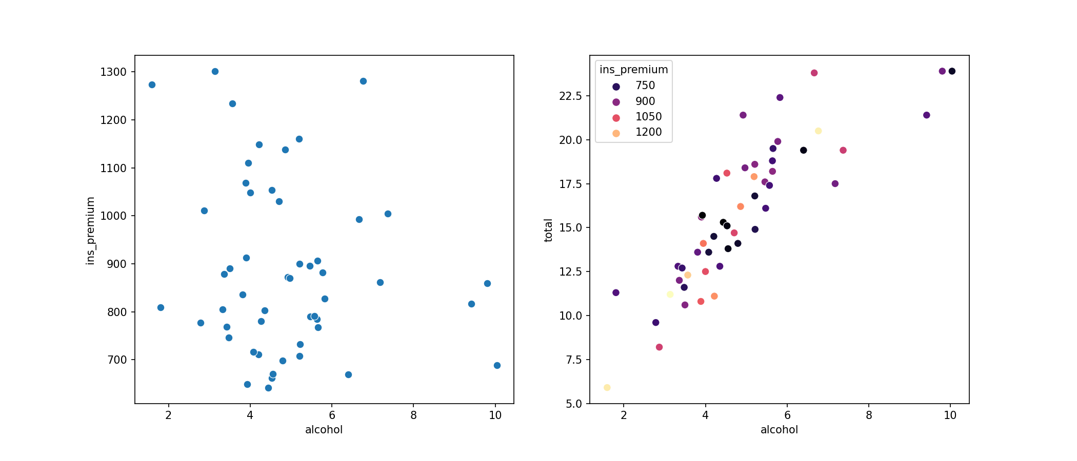
In the plot on the left, we can see that there isn't much of a relationship between our two independent variables: alcohol impairment and insurance premiums don't seem to have a strong correlation. On the plot on the right, we have our independent variable (alcohol) on the x-axis and the dependent variable (total) on the y-axis. We've chosen to plot the insurance premium variable (ins_premium) on the same axes but color-coded to visualize any correlations.
Now, let's fit the model with two independent variables.
import seaborn as sns
from statsmodels.formula.api import ols

crashes = sns.load_dataset("car_crashes")
model = ols('total ~ alcohol + speeding', data=crashes).fit()

print(model.summary())
                            OLS Regression Results
==============================================================================
Dep. Variable:                  total   R-squared:                       0.730
Model:                            OLS   Adj. R-squared:                  0.719
Method:                 Least Squares   F-statistic:                     64.87
Date:                Wed, 21 Apr 2021   Prob (F-statistic):           2.27e-14
Time:                        13:48:00   Log-Likelihood:                -110.71
No. Observations:                  51   AIC:                             227.4
Df Residuals:                      48   BIC:                             233.2
Df Model:                           2
Covariance Type:            nonrobust
==============================================================================
                 coef    std err          t      P>|t|      [0.025      0.975]
------------------------------------------------------------------------------
Intercept      5.6807      0.957      5.934      0.000       3.756       7.606
alcohol        1.9152      0.241      7.954      0.000       1.431       2.399
speeding       0.1502      0.206      0.728      0.470      -0.265       0.565
==============================================================================
Omnibus:                        2.495   Durbin-Watson:                   1.809
Prob(Omnibus):                  0.287   Jarque-Bera (JB):                2.045
Skew:                           0.490   Prob(JB):                        0.360
Kurtosis:                       2.978   Cond. No.                         23.5
==============================================================================

Notes:
[1] Standard Errors assume that the covariance matrix of the errors is correctly specified.
Now that we've added another variable, we have an additional line in our model for speeding, which includes the value of the coefficient.
Challenge
More variables could be added to this model! We still haven't explored the no_previous,
not_distracted, and ins_premium variables. Try adding a different variable in
place of
speeding and then look at the R-squared value. How does it change? In the next objective
in this module, we'll look more closely at the p-value and t-value.
Additional Resources
Objective 02 - Conduct a t-test to Determine the Significance of Individual Variables in the Model
Overview
Let's review:
- In the previous objective we
- added another variable to our linear regression
- restated the null hypothesis: slopes (Beta_1 and Beta_0) are both zero for both variables
- looked at the R-squared value
We have a good understanding of how to add another variable to linear regression. But we still have a few more things to look at in this analysis. Mainly - we're ready to perform a t-test on the additional variable in our regression model. So, how do we interpret the t-statistic and the resulting p-value with this new variable?
Again, we'll import our car crash data and fit a multiple linear regression model.
import pandas as pd
import seaborn as sns

# Load the car crash dataset
crashes = sns.load_dataset("car_crashes")

crashes.head()| total | speeding | alcohol | not_distracted | no_previous | ins_premium | ins_losses | abbrev | |
|---|---|---|---|---|---|---|---|---|
| 0 | 18.8 | 7.332 | 5.640 | 18.048 | 15.040 | 784.55 | 145.08 | AL |
| 1 | 18.1 | 7.421 | 4.525 | 16.290 | 17.014 | 1053.48 | 133.93 | AK |
| 2 | 18.6 | 6.510 | 5.208 | 15.624 | 17.856 | 899.47 | 110.35 | AZ |
| 3 | 22.4 | 4.032 | 5.824 | 21.056 | 21.280 | 827.34 | 142.39 | AR |
| 4 | 12.0 | 4.200 | 3.360 | 10.920 | 10.680 | 878.41 | 165.63 | CA |
# Import the OLS model from statsmodels
from statsmodels.formula.api import ols

# Set-up and fit the model in one step
# (format Y ~ X1 + X2)
model = ols('total ~ alcohol + speeding', data=crashes).fit()

# Print the model summary
print(model.summary())
                            OLS Regression Results
==============================================================================
Dep. Variable:                  total   R-squared:                       0.730
Model:                            OLS   Adj. R-squared:                  0.719
Method:                 Least Squares   F-statistic:                     64.87
Date:                Sat, 10 Oct 2020   Prob (F-statistic):           2.27e-14
Time:                        14:32:50   Log-Likelihood:                -110.71
No. Observations:                  51   AIC:                             227.4
Df Residuals:                      48   BIC:                             233.2
Df Model:                           2
Covariance Type:            nonrobust
==============================================================================
                 coef    std err          t      P>|t|      [0.025      0.975]
------------------------------------------------------------------------------
Intercept      5.6807      0.957      5.934      0.000       3.756       7.606
alcohol        1.9152      0.241      7.954      0.000       1.431       2.399
speeding       0.1502      0.206      0.728      0.470      -0.265       0.565
==============================================================================
Omnibus:                        2.495   Durbin-Watson:                   1.809
Prob(Omnibus):                  0.287   Jarque-Bera (JB):                2.045
Skew:                           0.490   Prob(JB):                        0.360
Kurtosis:                       2.978   Cond. No.                         23.5
==============================================================================

Warnings:
[1] Standard Errors assume that the covariance matrix of the errors is correctly specified.
Remember, in the previous objective, we considered that speeding might be a factor in the total number of accidents in which a driver is involved. So we added this variable to our regression model to test this out.
Well, our model says otherwise! If we look at the variable speeding, we can see that we have a p-value of 0.47. Recall that if the p-value is more significant than our critical value, we fail to reject the null hypothesis. In other words, we can't reject the statement that there is NO relationship between total accidents and speeding. So it seems that speed is not as big of a factor in accidents as we might have thought!
Let's look at the R-squared value: it was 0.727 for one variable (alcohol), and when we added a second variable (speeding), the adjusted R-squared went down. These results would suggest that the speeding variable didn't help to explain any additional variation in the target variable (total). Therefore, our interpretation of the p-value and the null hypothesis was correct.
We're going to look more closely at R-squared and adjusted R-squared in the next objective.
Challenge
As in the previous objective, we only looked at one additional variable. So go ahead and repeat the analysis above but try one of the other variables.
Additional Resources
Objective 03 - Compare Model Fit Using Adjusted R-squared
Overview
In the last two objectives, we learned how to add an additional variable to a linear regression model, perform a t-test, and interpret the p-value for the new variable.
Finally, we're going to look more closely at the R-squared and adjusted R-squared values. Specifically, we'll look at how they change from having one variable in our regression model and adding an additional variable.
As usual, we'll import the data and fit the model: first with just one variable (alcohol)
and again with the second variable (speeding).
import pandas as pd
import seaborn as sns

# Load the car crash dataset
crashes = sns.load_dataset("car_crashes")

crashes.head()| total | speeding | alcohol | not_distracted | no_previous | ins_premium | ins_losses | abbrev | |
|---|---|---|---|---|---|---|---|---|
| 0 | 18.8 | 7.332 | 5.640 | 18.048 | 15.040 | 784.55 | 145.08 | AL |
| 1 | 18.1 | 7.421 | 4.525 | 16.290 | 17.014 | 1053.48 | 133.93 | AK |
| 2 | 18.6 | 6.510 | 5.208 | 15.624 | 17.856 | 899.47 | 110.35 | AZ |
| 3 | 22.4 | 4.032 | 5.824 | 21.056 | 21.280 | 827.34 | 142.39 | AR |
| 4 | 12.0 | 4.200 | 3.360 | 10.920 | 10.680 | 878.41 | 165.63 | CA |
# Import the OLS model from statsmodels
from statsmodels.formula.api import ols

# Set-up and fit the model in one step
# (format Y ~ X)
model = ols('total ~ alcohol', data=crashes).fit()

# Print the model summary
print(model.summary())
                            OLS Regression Results
==============================================================================
Dep. Variable:                  total   R-squared:                       0.727
Model:                            OLS   Adj. R-squared:                  0.721
Method:                 Least Squares   F-statistic:                     130.5
Date:                Sat, 10 Oct 2020   Prob (F-statistic):           2.04e-15
Time:                        14:33:40   Log-Likelihood:                -110.99
No. Observations:                  51   AIC:                             226.0
Df Residuals:                      49   BIC:                             229.8
Df Model:                           1
Covariance Type:            nonrobust
==============================================================================
                 coef    std err          t      P>|t|      [0.025      0.975]
------------------------------------------------------------------------------
Intercept      5.8578      0.921      6.357      0.000       4.006       7.709
alcohol        2.0325      0.178     11.422      0.000       1.675       2.390
==============================================================================
Omnibus:                        1.922   Durbin-Watson:                   1.776
Prob(Omnibus):                  0.382   Jarque-Bera (JB):                1.705
Skew:                           0.439   Prob(JB):                        0.426
Kurtosis:                       2.824   Cond. No.                         16.2
==============================================================================

Warnings:
[1] Standard Errors assume that the covariance matrix of the errors is correctly specified.
# Set-up and fit the multiple regression model
# (format Y ~ X1 + X2)
model = ols('total ~ alcohol + speeding', data=crashes).fit()

# Print the model summary
print(model.summary())
                            OLS Regression Results
==============================================================================
Dep. Variable:                  total   R-squared:                       0.730
Model:                            OLS   Adj. R-squared:                  0.719
Method:                 Least Squares   F-statistic:                     64.87
Date:                Sat, 10 Oct 2020   Prob (F-statistic):           2.27e-14
Time:                        14:33:40   Log-Likelihood:                -110.71
No. Observations:                  51   AIC:                             227.4
Df Residuals:                      48   BIC:                             233.2
Df Model:                           2
Covariance Type:            nonrobust
==============================================================================
                 coef    std err          t      P>|t|      [0.025      0.975]
------------------------------------------------------------------------------
Intercept      5.6807      0.957      5.934      0.000       3.756       7.606
alcohol        1.9152      0.241      7.954      0.000       1.431       2.399
speeding       0.1502      0.206      0.728      0.470      -0.265       0.565
==============================================================================
Omnibus:                        2.495   Durbin-Watson:                   1.809
Prob(Omnibus):                  0.287   Jarque-Bera (JB):                2.045
Skew:                           0.490   Prob(JB):                        0.360
Kurtosis:                       2.978   Cond. No.                         23.5
==============================================================================

Warnings:
[1] Standard Errors assume that the covariance matrix of the errors is correctly specified.
Looking at the R-squared value for the model with one variable, we can see that alcohol explains 72.7% (0.727) of the variance in total accidents. When we add in speeding, though, the R-squared value increases to 0.730 but the adjusted R-squared value decreases from 0.721 to 0.719. R-squared values tend to increase with the number of variables added to our model, even if those variables are not useful in explaining the target any better. Adjusted R-squared values on the other hand, adds in a term to adjust for using multiple independent variables in linear regression. So, if R-squared does not increase significantly when we add the new variable(s), then the adjusted R-squared value will actually decrease.
The decrease is what happened here! We added in speeding, and the adjusted R-squared decreased. The result would imply that speeding doesn't help explain the variance in the target variable (total).
Challenge
This is your last chance to experiment with this multiple regression model (okay, not really - you have all the code and can run this model a million times if you like). But, you can now add different variables to the regression model and see if the R-squared and adjusted R-squared values increase.
Additional Resources
Guided Project
Open DS_132_Multiple_Regression.ipynb in the GitHub repository below to follow along with the guided project:
Guided Project Video
Module Assignment
Complete the Module 2 assignment to practice multiple regression techniques you've learned.