Module 4: Linear Correlation and Regression
Module Overview
In this module, we'll transition from hypothesis testing to understanding and quantifying relationships between variables. Linear correlation and regression are foundational statistical techniques used to measure the strength of relationships between variables and to build predictive models.
These methods allow us to answer questions like: How strongly are two variables related? Can we use one variable to predict another? Is there a meaningful linear relationship between variables? These are crucial skills for data scientists, as they form the basis for more advanced predictive modeling techniques.
Learning Objectives
- Distinguish between independent and dependent variables
- Distinguish between linear and non-linear relationships
- Calculate the linear correlation using the scipy.stats library
- Calculate and interpret the slope and intercept
- Calculate a prediction and a residual
Objective 01 - Distinguish Between Independent and Dependent Variables and Connect With the Terms Features and Target
Overview
In this module, we are going to learn how to measure the linear relationship between quantitative variables. A quantitative variable usually measures something, such as counts, percents, numbers, and dates. It can take on a range of values.
When we want to determine a relationship between variables, we'll often plot them on a scatter plot. In this objective, we'll learn how to distinguish between independent variables and dependent variables.
Visualize the Data
Let's look at some data to get started. This data set is available from the UCI Machine Learning Repository. It contains information about how the compressive strength of concrete depends on the different properties of the mixture.
We will use this data throughout this module to learn how to identify dependent and independent variables.
Let's go ahead and load in the data to get started.
import pandas as pd

url = 'https://raw.githubusercontent.com/bloominstituteoftechnology/data-science-practice-datasets/main/unit_1/Concrete/Concrete_Data.csv'

concrete = pd.read_csv(url)

concrete.head()| cement | furnace | fly_ash | water | super_plasticize | coarse_agg | fine_agg | age | strength | |
|---|---|---|---|---|---|---|---|---|---|
| 0 | 540.0 | 0.0 | 0.0 | 162.0 | 2.5 | 1040.0 | 676.0 | 28 | 79.99 |
| 1 | 540.0 | 0.0 | 0.0 | 162.0 | 2.5 | 1055.0 | 676.0 | 28 | 61.89 |
| 2 | 332.5 | 142.5 | 0.0 | 228.0 | 0.0 | 932.0 | 594.0 | 270 | 40.27 |
| 3 | 332.5 | 142.5 | 0.0 | 228.0 | 0.0 | 932.0 | 594.0 | 365 | 41.05 |
| 4 | 198.6 | 132.4 | 0.0 | 192.0 | 0.0 | 978.4 | 825.5 | 360 | 44.30 |
All of these variables are numeric, so we have some choices. We'll start by looking at the amount of
cement in the concrete mixture (cement) and the compressive strength of the cement
(strength). When we create a plot, we need to choose which axis to plot each variable. So,
how do we decide?
As you can see in the DataFrame, we have several columns containing physical measurements of the
concrete, such as water content, the number of different aggregates, and even the age. But one of the
columns is different: the concrete's compressive strength (strength) depends on all of
these other measurements.
In this case, we state that the cement content is the independent variable, and the strength is the dependent variable. When we create a two-dimensional plot, the independent variables go on the x-axis and the dependent variable on the y-axis.
Let's look at our plot.
# Create the visualization

import matplotlib.pyplot as plt

plt.scatter(x=concrete['cement'], y=concrete['strength'])
plt.xlabel('Cement content (kg/cubic meter)')
plt.ylabel('Compressive strength')
plt.title('Concrete Properties')

#plt.show()
plt.clf()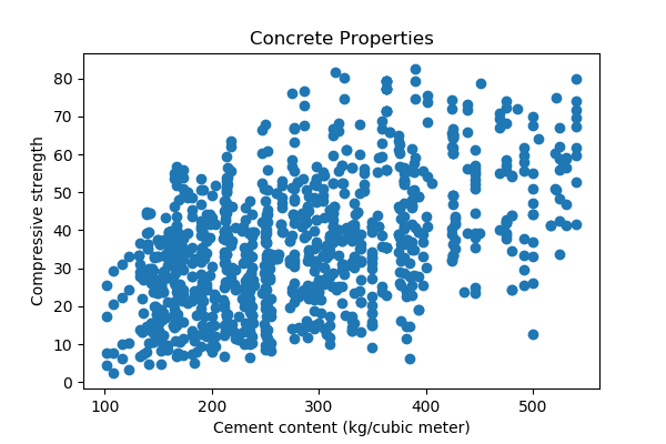
In the plot above, we can see a relationship (even a slight one) between our two variables. For example, we could state it like this: as the cement content increases, the compressive strength of the concrete also increases. We'll come back to this type of relationship later in the module. But first, let's go back to the dependent and independent variable terms.
Independent and Dependent Variables
In our plot, the compressive strength is the dependent variable. It changes when the other variables change, such as the cement content. Therefore, dependent variables are the target when we discuss predictive models. In other words, the target is what we're trying to predict.
And because the amount of cement is the quantity we control and can change in our data collection, this
variable is referred to as the independent variable. In predictive modeling, these
variables are features. We use the features to predict the target. For example, we have
one feature (cement) and one target (strength) in the data plotted above.
Let's consider a few other datasets and identify the dependent and independent variables.
Follow Along
Consider the following situations (try to identify the dependent/independent variables before reading the answer):
- You measure how the amount of sugar affects the taste of coffee. What are the dependent and independent variables? (In this case, we change the amount of sugar (independent) and measure how it affects taste (dependent)).
- You would like to examine medication dosage and the severity of specific symptoms. What are the dependent and independent variables? (The dosage is the independent variable, and the symptom severity is dependent on the dosage).
-
And the final problem (this one might be a little trickier):
You have measurements for the amount of a particular compound in the atmosphere and the average global temperature record for many thousands of years. What are the dependent and independent variables here? (The temperature depends on the amount of the compound. Even though we can't change the atmospheric composition in our observational study, it is the independent variable).
Challenge
You're probably already familiar with the UCI Machine Learning Repository. Right now would be an excellent time to explore the available datasets for this challenge. You can even select the types of problems (regression, classification) you would use to filter your datasets. Select a few datasets, read over the descriptions, and identify the dependent/independent variables. The variables will often be the features and target, so pay attention to that wording.
Objective 02 - Distinguish Between Linear and Nonlinear Relationships on a Scatterplot and Calculate a Linear Correlation
Overview
In the first part of the module, we introduced independent and dependent variables and practiced identifying them in different datasets. We also looked at a scatterplot of a dataset to illustrate which axis to plot the dependent and independent variables.
Now, we're going to look more closely at the data and any patterns or correlations between the variables. Again, visualizations like scatterplots are a great way to plot a few variables and see any correlations.
Correlation
In general, correlation is a statistical term that describes the relationship between two random variables. But correlation, as used in the term linear correlation, is the degree to which two variables are linearly related. In other words, when we plot two variables on a scatterplot, could we draw a line through the data in any direction? If we draw a line, the resulting slope can tell us how the two variables are correlated.
Degree of Correlation
We can measure how well two variables are correlated. This measurement ranges between -1 and 1:
- -1: Two variables are negatively correlated where an increase in one results in a decrease in the other
- 0: There is no linear relationship between two variables (though they can have a non-linear relationship)
- +1: Two variables are positively correlated where an increase in one increases the other
Follow Along
Let's look at the concrete strength dataset from the previous objective. We don't need to use all of the columns, so we'll only load some features. Having looked at the data previously, we can see that some variables are correlated more closely than others. So, we'll select cement, water, course_agg, and strength for the following analysis.
import pandas as pd

url = 'https://raw.githubusercontent.com/bloominstituteoftechnology/data-science-practice-datasets/main/unit_1/Concrete/Concrete_Data.csv'

# Use these columns:
mycols = ['cement', 'water','coarse_agg', 'strength']
concrete = pd.read_csv(url, usecols=mycols)
Now, let's create a pair plot! The seaborn plotting library has a particular type of plot called a pair plot: we can look at pairs of variables on a grid of scatter plots. It's a convenient way to quickly look at your data and identify any characteristics or correlations you would like to explore further.
import matplotlib.pyplot as plt
import seaborn as sns

sns.pairplot(concrete)

plt.savefig('/Users/nicole/data_science_LS/data-science-canvas-images/unit_1/sprint_3/new/mod1_obj2_concrete_pair.png',
            transparent=False, dpi=100)

plt.show()
plt.clf()
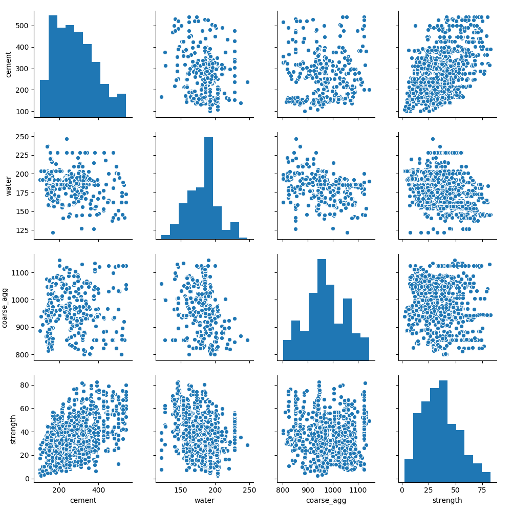
In the plot above, we can see our four features and how they correlate with each other. We'll choose two of these features and calculate the correlation between them. First, we'll look at these features: the strength and cement content (cement) and the strength and water content (water).
To find the correlation between our variables, we'll calculate the Pearson correlation coefficient. Calculating the Pearson correlation is determined by finding the covariance of the two variables and dividing by the product of the standard deviation of each data sample. In other words, we are calculating the normalization of the covariance between the two variables.
from scipy.stats import pearsonr

# Calculate the correlation coefficient
# (return only the coefficient)
strength_cement, _ = pearsonr(concrete['strength'], concrete['cement'])
strength_water, _ = pearsonr(concrete['strength'], concrete['water'])

print('The correlation between strength-cement:', round(strength_cement, 3))
print('The correlation between strength-water:', round(strength_water, 2))
The correlation between strength-cement: 0.498
The correlation between strength-water: -0.29
In this example, we see a positive correlation between concrete strength and cement content - as the cement increases, the strength of the concrete increases. On the other hand, as the water content increases, the strength of the cement decreases, as indicated by the negative correlation coefficient.
Challenge
There are still several sets of variables for which we haven't calculated the correlation. Following the same steps as above, calculate the correlation coefficients for some of those variables. To challenge yourself, look at the pair plot or scatterplot first, and predict if the correlation is positive or negative.
Additional Resources
Objective 03 - Calculate and Interpret the Slope and Intercept of a Simple Linear Regression Model and Make a Prediction
Overview
In this module so far, we've explored dependent/independent variables, created scatter plots, and calculated linear correlations for sets of variables. Now we're going to learn how to fit our first model to data: a linear regression. Regression is a statistical method for determining the relationship between variables. Linear regression is the process of finding a line that best fits a given set of data.
Ordinary Least Squares
So how do we find this line? The method of ordinary least squares (OLS)! Right now, we'll stick to a relatively simple explanation and save the derivations and the discussion of how this method works for later in the course (or even self-study - see the Additional Resources section at the bottom for more information).
The ordinary least squared method finds a best-fit line by finding the parameters for the line equation that minimizes the error square.
Linear Equations
One of the most common ways to represent a line is with the equation
y = mx + bwhere x is our independent variable (or feature) and y is the dependent variable (or target). The value of m is the slope of the line and b is the intercept.
But we're going to use a different more general notation, using the letter b (sometimes this term is a beta or β).
y = b0 + b1xwhere b0 is now the intercept and b1 is the slope. The x and y variables are still the same as above; we've only changed the constants. You may see a slightly different representation in the Guided Project - don't panic! Look carefully at each equation and identify what looks different. This is also part of learning math and being comfortable using it in data science applications.
Let's look at a plot of a line and identify the slope and intercept. Then we'll move onto some real data and fit a line.
# Import the predictor class

from sklearn.linear_model import LinearRegression

# Instantiate the class (with default parameters)

model = LinearRegression()

# Assign the data to the x and y variables (easier to see what we are fitting)

x = concrete['cement']

# Add a new axis to create a column vector

# (scikit-learn expects the data to be in this shape)

X = np.array(x)[:, np.newaxis]

y = concrete['strength']

# Fit the model - so exciting!

model.fit(X, y)
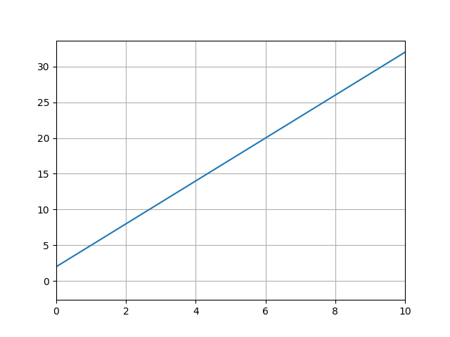
In the plot, we can see the intercept is two and the slope is equal to three. The slope is the change in y over the change in x; from the plot we can do a quick calculation: (change_y/change_x) = (20-2)/(6-0) = 18/6 = 3.
We didn't fit any data to a line yet, so follow along in the next section while we implement a linear regression.
Follow Along
- load in the concrete data
- fit a linear regression
- look at the coefficients
- make a prediction
We'll use the concrete strength data set again and fit a linear regression to the concrete strength
(strength) and cement content (cement). We'll read in the whole dataset, in
case we'd like to use more than one feature to fit a linear regression.
import pandas as pd

url = 'https://raw.githubusercontent.com/bloominstituteoftechnology/data-science-practice-datasets/main/unit_1/Concrete/Concrete_Data.csv'

concrete = pd.read_csv(url)

concrete.head()| cement | furnace | fly_ash | water | super_plasticize | coarse_agg | fine_agg | age | strength | |
|---|---|---|---|---|---|---|---|---|---|
| 0 | 540.0 | 0.0 | 0.0 | 162.0 | 2.5 | 1040.0 | 676.0 | 28 | 79.99 |
| 1 | 540.0 | 0.0 | 0.0 | 162.0 | 2.5 | 1055.0 | 676.0 | 28 | 61.89 |
| 2 | 332.5 | 142.5 | 0.0 | 228.0 | 0.0 | 932.0 | 594.0 | 270 | 40.27 |
| 3 | 332.5 | 142.5 | 0.0 | 228.0 | 0.0 | 932.0 | 594.0 | 365 | 41.05 |
| 4 | 198.6 | 132.4 | 0.0 | 192.0 | 0.0 | 978.4 | 825.5 | 360 | 44.30 |
We're going to use the scikit-learn library LinearRegression() model to find our best-fit
line. You will be working with this library extensively in future sprints, so don't worry if it seems
confusing at first. Just pay attention to the comments in the code and then look at how we pull the
slope and intercept from the results of the model.
# Import the predictor class
from sklearn.linear_model import LinearRegression

# Instantiate the class (with default parameters)
model = LinearRegression()

# Assign the data to the x and y variables (easier to see what we are fitting)

x = concrete['cement']
# Add a new axis to create a column vector
# (scikit-learn expects the data to be in this shape)
X = x[:, np.newaxis]

y = concrete['strength']

# Fit the model - so exciting!
model.fit(X, y)
LinearRegression(copy_X=True, fit_intercept=True, n_jobs=None, normalize=False)
Cool! Now, we'll pull the slope and intercept parameters out of the model that we fit.
# Slope (also called the model coefficient)
print('The slope: ', model.coef_)

# Intercept
print('The intercept: ', model.intercept_)

# In equation form
print('Best-fit line: y = {:.2f}x + {:.2f}'.format(model.coef_[0], model.intercept_))
The slope:  [0.07958034]
The intercept:  13.44252811239992
Best-fit line: y = 0.08x + 13.44
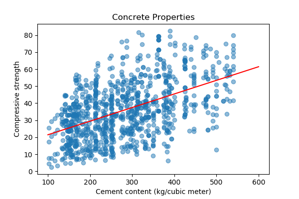
We'll now plot the data and the best-fit line.
import matplotlib.pyplot as plt

# Plot the data
plt.scatter(x=x, y=y, alpha=0.5)

# Plot the best-fit line
x_bestfit = np.linspace(100, 600, 10)
y_bestfit = 0.08*x_bestfit + 13.44
plt.plot(x_bestfit, y_bestfit, color='red')

plt.xlabel('Cement content (kg/cubic meter)')
plt.ylabel('Compressive strength')
plt.title('Concrete Properties')

#plt.show()
plt.clf()
<Figure size 432x288 with 0 Axes>
Making a Prediction
We're finally at the fun part: making predictions with our model. In the above example, where we fit a linear regression model to our concrete data, we might want to use our results to make a prediction. Now, there isn't a very strong correlation between cement content and the strength of concrete. But, we can still make a prediction with our results.
We'll select a value of our independent variable (cement content) and predict the strength. Let's choose cement=600 and plug it into our equation for the best-fit line:
We can read this value off the graph, as expected. In the next module, we'll talk about the statistics of making predictions from our models.
Challenge
Now it's your turn! First, you can look at one of the other variables, like water content
(water), and fit a linear regression model. Then plot the line along with your data. Are
the slope and intercept parameters different?
Additional Resources
Objective 04 - Calculate a Residual
Overview
In this module so far, we've covered the basics of identifying dependent and independent variables, calculating correlation, fitting a linear regression model, and making a prediction. Now, we're going to introduce the concept of a residual.
When we make a prediction, we then have predicted values. But remember, there are also the observed values. A residual is a difference between the predicted value and the observed value for a given data point.
To determine the parameters when fitting a linear model, we want to minimize the residuals. In other words, when we sum up all of the residuals for all of the data points, we want to find the slope and intercept that results in the smallest residual.
Follow Along
Using the concrete strength example from the previous objectives, let's calculate the residual for one of the data points.
import pandas as pd

url = 'https://raw.githubusercontent.com/bloominstituteoftechnology/data-science-practice-datasets/main/unit_1/Concrete/Concrete_Data.csv'

concrete = pd.read_csv(url)

concrete.head()| cement | furnace | fly_ash | water | super_plasticize | coarse_agg | fine_agg | age | strength | |
|---|---|---|---|---|---|---|---|---|---|
| 0 | 540.0 | 0.0 | 0.0 | 162.0 | 2.5 | 1040.0 | 676.0 | 28 | 79.99 |
| 1 | 540.0 | 0.0 | 0.0 | 162.0 | 2.5 | 1055.0 | 676.0 | 28 | 61.89 |
| 2 | 332.5 | 142.5 | 0.0 | 228.0 | 0.0 | 932.0 | 594.0 | 270 | 40.27 |
| 3 | 332.5 | 142.5 | 0.0 | 228.0 | 0.0 | 932.0 | 594.0 | 365 | 41.05 |
| 4 | 198.6 | 132.4 | 0.0 | 192.0 | 0.0 | 978.4 | 825.5 | 360 | 44.30 |
Using the fifth data point (index 4), we'll plug the cement content value of 198.6 into our linear regression equation. Recall the parameters for the best-fit line are:
where y is the predicted concrete strength and x is the cement content. Substituting into our equation gives us:
The observed strength value for this cement content was 44.3, so the residual is 44.30-29.3 = 15.
Not all residuals will be positive or even very large - some will be negative, and some will be very small and close to the prediction. The sum of the squares of all residuals is the crucial value and what we minimize when fitting a linear regression model.
Challenge
Using the same dataset, look through the DataFrame to find another data point to calculate the residual. Can you find one that is very close to the prediction, with a slight residual? How about an observation that has a large residual?
Additional Resources
Guided Project
Open DS_124_Simple_Linear_Regression.ipynb in the GitHub repository below to follow along with the guided project:
Guided Project Video
Module Assignment
Complete the Module 4 assignment to practice linear correlation and regression techniques you've learned.