Module 1: Hypothesis Testing (t-tests) and Confidence Intervals
Module Overview
In this module, we're going to build on the descriptive statistics concepts we've already learned about as we started to explore our data. This module will introduce the idea of a "hypothesis test" and how we implement one, specifically using the t-test and t-distributions. We'll also cover how to calculate p-values and use the results to interpret our hypothesis.
In addition, this module will cover one of the most important concepts in statistics: the Central Limit Theorem. We'll learn about the properties of sampling distributions and how to interpret the expected mean of a sample distribution, which will, in turn, lead to the idea of confidence intervals and how we know the confidence level of our results and predictions.
Learning Objectives
- Explain the Purpose of a t-test and Identify Applications
- Set up and run one-sample and two-sample t-tests
- Draw conclusions with null and alternative hypotheses
- Explain the concepts of statistical estimate, precision, and standard error as they apply to inferential statistics
- Explain the implications of the central limit theorem in inferential statistics
- Explain the purpose of and identify applications for confidence intervals
Objective 01 - Explain the Purpose of a t-test and Identify Applications
Overview
Before we learn about t-tests, we should cover some more basic information about the concept of hypothesis testing first. When interpreting our data or results, we want to confirm or reject an assumption about that data or result. This assumption can also be called a hypothesis. So, before we interpret our results (hopefully), we will have stated our hypothesis. Then, we need to test it to determine at what confidence level we know our results. Hypothesis tests are also known as significance tests, meaning we want to know how significant our result is.
When we use statistical methods to test our hypothesis, we're conducting a statistical hypothesis test. There are several different statistical tests we can do. For this objective, we're going to be focusing on t-tests. They make use of a statistical distribution called the Student's t-distribution.
But, before we get into the t-distribution, a refresher of the normal distribution will be helpful.
Normal distribution
The normal probability distribution comes up very frequently in the study of probability and statistics. A variable that has a normal distribution is one where the mean = median = mode. A normal distribution is theoretical, which means that in nature, nothing will strictly follow this distribution. But many variables approximate to it, such as the height of adult humans, birth weight of human babies, height of the same variety of pine trees.
The normal distribution is known as a bell curve because it has the shape of a bell. Using the numpy normal distribution, we can draw a sample population with a specified mean (center point of the "bell") and standard deviation (width or "spread" of the curve), and plot it.
import seaborn as sns
import matplotlib.pyplot as plt

# The mean of a normal distribution can be any value
# (we're using 0 for plotting nicely and to see the symmetry)
mean = 0

# The width of the normal distribution is set by the standard deviation
sigma = 1

# Create a sample drawn from the normal distribution
sample = np.random.normal(loc=mean, scale=sigma, size=1000)

# Create the fig and axes object and plot
fig, ax = plt.subplots(figsize=(8,8))
ax = sns.displot(sample)
ax.set_titles('The normal distribution', fontsize=16)

fig.clf()
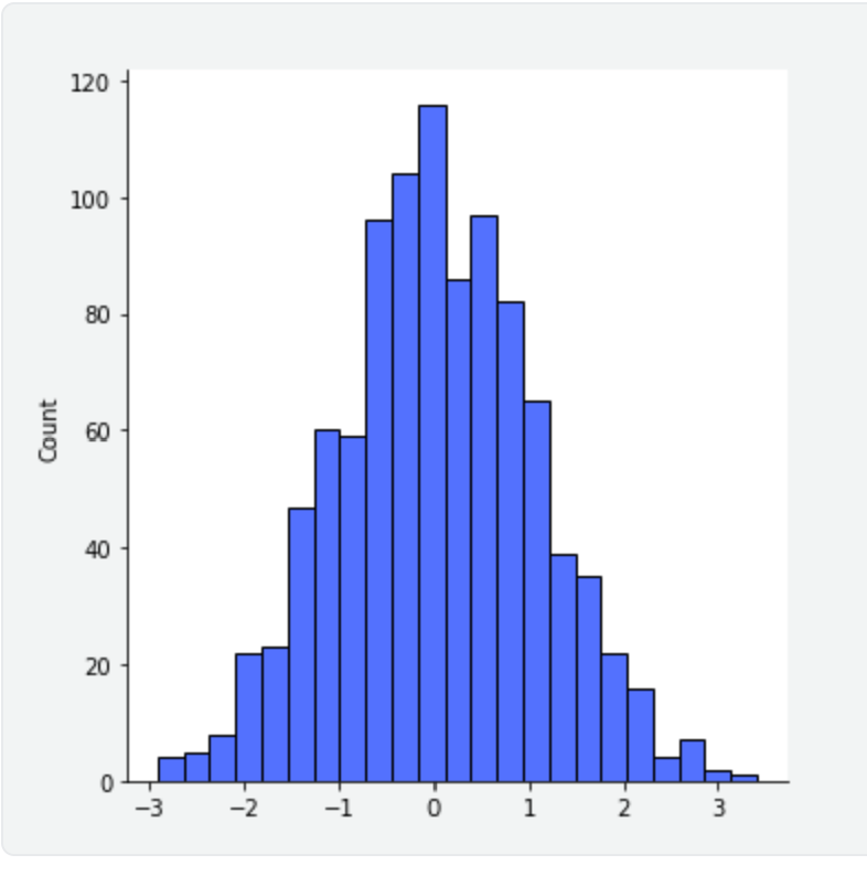
In the plot, we can see a nice bell shape, centered on the mean we specified as 0 and with a standard deviation of the sample equal to 1.
The z-score
In statistics, we also use something called the z-score. Say, for example, you take a value at random from the distribution above. We can calculate a z-score for that value which describes its position in terms of the distance from the mean when measured in standard deviation units. Z-scores may be positive or negative, with a positive value indicating the score is above the mean and a negative score below the mean. For example, a z-score of 1 means the value you chose is one standard deviation from the mean.
The t-values and t-tests
In some situations, we have to draw a sample from a population whose mean is unknown. What if for the normal distribution plotted above, and we had set the mean equal to one?
In such scenarios, we use the sample's mean instead. When we use the mean of the sample and not the mean of the population from which we drew the sample, we calculate the t-value. This value is similar to the z-score but we use the mean of the sample instead of the population to calculate it.
A t-test is based on a t-value. When you perform a t-test for a single study, you obtain a single t-value. If you drew lots of random samples of the same size from the same population, performed a t-test each time (to obtain a t-value), you could then plot a distribution of all the t-values. This type of distribution is called a sampling distribution and, in this case, a t-distribution.
Thanks to math and statisticians, the properties of t-distributions are well understood, so we can plot them without having to draw samples, calculate the t-value, etc. A specific t-distribution is defined by its degrees of freedom (dof), with a sample size-1. So there is a whole "family" of t-distributions for every sample size. For large samples size (n > 120), the shape of the t-distribution is almost identical to the normal distribution. For smaller sample sizes, the t-distribution is much flatter in the middle. In the next section, we'll look at the t-distribution graphically.
When to use a t-test?
There are a few situations where using a t-test is useful. In this lesson, we will be focusing on two:
One-sample t-test
One of the most common one-sample t-tests is to determine the statistical difference between a sample mean and a known or hypothesized value of the mean in the population. For example, say we want to compare the average Netflix watching time for a specific group of viewers, such as ages 5-12 (mean value of the sample), and compare it to the average Netflix time for the US population (mean value for the population from the sample ). Then, we perform a t-test to determine how effective the mean of the sample is in comparison to the general population - does this age group watch significantly more or less Netflix? Or is it not statistically different?
Two-sample t-test (also called an independent t-test)
A two-sample t-test is helpful if we want to compare the mean of two samples and determine if a property is true. example, say you want to know if the mean petal length of iris flowers differs according to their species. So you measure 25 petals of each species and then test the difference between these two groups using a t-test.
Follow Along
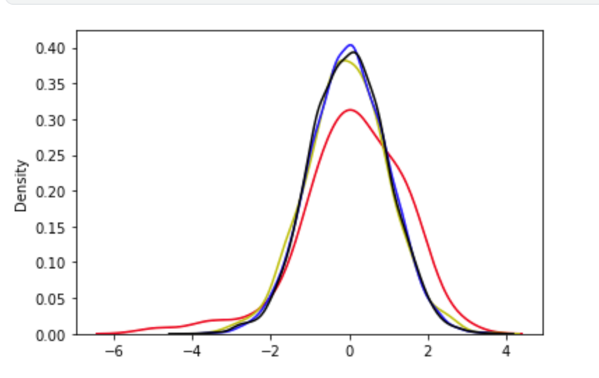
We've covered the concepts of distributions and t-values. Now, we can look at some graphical representations of these distributions. In the following plot, we created t-distributions with varying degrees of freedom. We can see that the t-distribution with the smallest number of degrees of freedom is flatter in the middle and "wider" on the sides. As the sample size increases (degrees of freedom increase), the t-distribution approaches the normal distribution (plotted in black).
# Import the libraries
import numpy as np
import matplotlib.pyplot as plt
import seaborn as sns

# Create the t-distributions
t_df10 = np.random.standard_t(df=10, size=100)
t_df100 = np.random.standard_t(df=100, size=1000)
t_df1000 = np.random.standard_t(df=1000, size=10000)

# Create the normal distribution
s = np.random.normal(size=10000)

# Create the figure and axes objects and plots
fig, ax = plt.subplots(1)

# Plot t-distributions
ax = sns.kdeplot(t_df10, color='r');
ax = sns.kdeplot(t_df100, color='y');
ax = sns.kdeplot(t_df1000, color='b');

# Plot normal distributions
sns.kdeplot(s, color='k');
Additional Resources
Objective 02 - Set Up and Run a one-sample or two-sample t-test
Overview
We've already reviewed the normal distributions and the t-distributions and how they are related to t-tests and t-values. Now we'll work through an example of a one-sample t-test where we calculate the t-value.
When we do a one-sample t-test, we're comparing the mean of our sample data to a known value. For example, we can look at the effectiveness of a cardio-based fitness program on cardiovascular health. We might sample a group of 50 individuals who participated in a program to lower their heart rate. After six months of the program, measurements were taken, and the mean heart rate was recorded. We would then like to compare the mean heart rate to the general US population. We'll look at the specifics in the next section and calculate the t-value, both by "hand" and using Python tools.
Follow Along
We'll expand slightly on the above example to calculate the t-value by hand (we'll write out the equation and work through each step). Then, we will compare that result to the calculation determined by using the SciPy stats module.
We will use SciPy and NumPy to draw a sample from a distribution. We will determine the mean and standard deviation from that sample, and then verify the t-value by hand.
Sample Information
The sample population we have consists of 50 individuals, with a mean heart rate of 69 beats per minute (bpm) and a standard deviation of 6.5 bpm. We'd like to compare this to the population mean heart rate of 72 bpm.
Calculate with Numpy and SciPy
# Import the stats module
from scipy import stats

# Generate the random test scores with the specified mean, std, and sample size
rvs = stats.norm.rvs(loc=69, scale=6.5, size=50, random_state=42)

# Display the test scores, as a check
rvs

# Check the sample mean and std
print('The mean of the sample: ', rvs.mean())
print('The standard deviation of the sample: ', rvs.std())

# Calculate the t value using the ttest_1samp
stats.ttest_1samp(rvs, popmean=72)
The mean of the sample:  67.53441961583509
The standard deviation of the sample:  6.00785209617076


Ttest_1sampResult(statistic=-5.2030346601039055, pvalue=3.841987344207577e-06)
Manual Calculation
We can see that the actual values for our sample distribution are slightly different. The difference is
because we're drawing a random distribution from the sample with stats.norm.rvs(). Using
the mean and standard deviation printed out from this random sample, we can verify the t-statistic by
hand.
The t-value is calculated by taking the following equation:
t-value = (sample mean-population mean) / standard error.
t-value = (67.53 - 72) / (6.01/sqrt(50))
For this example, we'll use Python's calculator abilities to do the math for us.
# Import the library
import numpy as np

# Calculate the t-value
tstatistic = (67.53-72)/(6.01/np.sqrt(50))
print('The t-statistic is: ', tstatistic)
The t-statistic is: -5.259180219473988They agree! It's an excellent exercise to write this out by hand so that you can better understand how we use the variables in the equations.
It's important to note that we can see both the t-statistic and p-value displayed. We'll cover the p-value and how to interpret it later in this module; for now, we'll focus on the t-statistic.
Challenge
Following the same example as above, generate a random distribution using the
stats.norm.rvs() method. Change the values of "loc" (mean) and "scale" (standard deviation)
and the sample size. Consider using some of the following variations:
- have the mean remain the same but change the "scale" (standard deviation)
- change the sample size("size") and see how it affect the t statistic
Additional Resources
Objective 03 - Set Up and Run a Two-sample Independent t-test
Overview
We've already reviewed normal and t-distributions, and calculated the t-statistic for one sample. Next, we'll work through an example for a two-sample t-test and then calculate the t-value for two independent populations.
When we do a one-sample t-test, we're comparing the mean of our sample data to a known value. For two-sample t-tests, to determine the t-value, you compare the means of two independent samples to a given variable. Expanding on our example from the one-sample test, we'll add another group of individuals participating in an exercise program to decrease their heart rate.
In other words, we'll compare the mean heart rate of the exercise group participating in a cardio-heavy program and another sample group participating in a yoga-based fitness program. The other parameters are the same: duration (six months), size of each sample population (50).
For a two-sample t-test, we want to know the average difference between the mean heart rates, if we repeatedly selected heart rate samples for each group of fitness participants.
Follow Along
For the two-sample t-tests, it's more challenging to calculate the t-value by hand; the equation is a little longer, and it's more involved when the sizes and variance/standard deviation are different for the two samples. So we'll use the power of Python!
Calculate with NumPy and SciPy
Here are the parameters we are using for our two-sample t-test:
- cardio-based program: mean=69 bpm, std=6.5 bpm
- yoga-based program: mean=71 bpm, std=7.3 bpm
Let's use some NumPy and SciPy tools to generate a normal distribution with the specified parameters. We have the sample means and sample standard deviations. We'll create a distribution of random variables with the given mean (loc) and standard deviation (scale).
# Import the libraries

import numpy as np

from scipy import stats
#apply a seed value that ensures that different machines will return the same result
np.random.seed(42)

# Generate the random variables with the specified mean, std, and sample size
#cardio
rvs1 = stats.norm.rvs(loc=69, scale=6.5,size=50)

#yoga
rvs2 = stats.norm.rvs(loc=71, scale=7.3, size=50)

# Calculate the t statistic for these two sample populations
stats.ttest_ind(rvs1, rvs2)
Ttest_indResult(statistic=-2.886610676042845, pvalue=0.004790856010749188)
Challenge
Using the same process as above, generate additional distributions with the specified mean and standard deviation and calculate the t-statistic for each set of populations. Consider using some of the following variations:
- have the mean remain the same but change the "scale" (standard deviation)
- change the sample sizes for each sample ("size") and see how it affect the t-statistic
Additional Resources
Objective 04 - Use a t-test p-value to Draw a Conclusion About the Null and Alternative Hypothesis
Overview
When we want to determine if a result is statistically significant, we need a standard to judge the hypotheses. For example, let's say we wanted to know if cardiovascular exercise can lower resting heart rate.
We could state our hypothesis that the mean resting heart rate in cardiovascular exercise individuals is not different from the mean resting heart rate for all US adults (78 beats per minute).
The process of this set of hypotheses might look something like the following:
- First, we state our null hypothesis: The mean heart rate in individuals who do cardiovascular exercise is not different from the mean heart rate of the rest of the population (78bpm).
- Second, we determine the alternative hypothesis: The mean heart rate in individuals who do cardiovascular exercise is different from the mean heart rate in the rest of the population (78bpm).
- We select a representative sample of cardiovascular exercise individuals and calculate the mean and SD heart rate.
The null hypothesis is written out symbolically as:
H_{0}: μ = reference valuewhere μ is the population mean of all individuals doing cardiovascular exercise.
In this specific situation:
H_{0}: μ = 78Although we suspect that cardiovascular exercise will lower resting heart rate, it is better to be "conservative" and use a "not equal to" alternative hypothesis is:
This is written symbolically as: H_{a}: μ != 78
Interpret the p-value
Now that we have decided on both the null and alternative hypotheses, we need to determine if we reject or fail to reject the null hypothesis. Here is where the p-value finally comes in. The p-value is the probability of observing our sample mean if the null hypothesis is true. We'll add to the hypothesis testing process from above:
- Decide on the null and alternative hypotheses.
- Determine the significance level you wish to use. Often this is 0.05, but it doesn't have to be.
- Calculate the test statistics (in this module, we have focused on the t statistic) and the associated p-value.
- Use the p-value and the significance level to determine if you reject or fail to reject the null hypothesis.
A note on the significance level: This value is also called the alpha level. If we choose alpha=0.05 or 5%, we would expect to incorrectly reject the null hypothesis 5% of the time. A stricter significance level of alpha=0.01 (1%) would mean that we would only expect to incorrectly reject the null hypothesis 1% of the time (also referred to as a Type 1 error). To reject the null hypothesis, the p-value needs to be less than the (alpha):
- p-value < alpha: reject the null hypothesis
- p-value > alpha: fail to reject the null hypothesis
We never accept a null hypothesis or prove it to be true, we can only fail to reject it.
In other words, failing to reject the null hypothesis means that we do not have enough evidence to conclude that the null hypothesis is false.
Follow Along
We want to test if a new method of teaching physics increases understanding as measured by higher scores on a particular physics test. Therefore, a random sample of 50 students who have learned using this new method is selected, and the mean score on the physics test is determined to be 74.6 with a standard deviation of 12.3.
We then want to compare this to the entire population of physics test scores, where the mean is 67.5.
The null hypothesis is that the mean tests score for students who learned using the new method is
equivalent to the mean test score for the entire population of physics students. We write this
symbolically as H_{0}: μ = 67.5
To be conservative, we won't automatically believe that the new method improves scores and will instead
specify that the alternative hypothesis is that the scores are simply not equal to each other
H_{a}: μ \neq 67.5.
Calculate with SciPy
Using the tools available in SciPy, we'll create random test scores for the general student population, with the given mean of 67.5. From this distribution, we'll select 50 scores with a mean of 74.6 and a standard deviation of 12.3. Using these values, we'll let SciPy calculate the t-statistic and p-value.
# Import the stats module
from scipy import stats

# Here are the 50 scores from the class (they were generated to have the correct mean and SD)
rvs = stats.norm.rvs(loc=74.6, scale=12.3, size=50, random_state=42)

# Calculate the t statistic and the p-value
stats.ttest_1samp(rvs,67.5)
Ttest_1sampResult(statistic=2.6640411076902604, pvalue=0.010421324745517498)
Interpret the p-value
We have a p-value of 0.0104. Let's compare this to the alpha value: p-value 0.0104 < 0.05. Therefore, we should reject the null hypothesis and conclude that students using the new method to learn physics do have a statistically significant mean physics test score compared to the entire population of physics students.
Additional Resources
Objective 05 - Explain the Concepts of Statistical Estimate, Precision, and Standard Error as They Apply to Inferential Statistics
Overview
So far, we have worked through several examples of hypothesis testing using t-tests in this course. In some of the equations we've worked with, we have used the standard error value (or the standard deviation). But we haven't covered what this standard error is. Once we better understand this concept, many of the other concepts we have used so far will make more sense. Statistics is often about understanding more straightforward concepts and then fitting them together into a larger conceptual framework.
Error
Most people are familiar with the concept of an error as used outside of statistics. For example, an
error can be a typo, an incorrect variable in an equation, or a bug in your Python code that results in
a TypeError or AssertionError. But what does the error mean as used in
statistics?
We have been working with this idea so far without really knowing it. In statistics, error refers to the random variation when we are drawing random samples from a distribution. In other words, it's not an unintentional mistake but another way to describe the variation in the parameters we are trying to measure.
We have been working with the mean values of populations from which we have gathered samples throughout this sprint. Since we're trying to understand the mean error for these sampling distributions, we're working with the standard error of the mean.
Expected value
Let's try to look at this another way. When we sample from a population, we calculate the mean of that sample. Then, when we sample from that population again, we get different values, which can (and usually do) have a different mean. So if we took 1000 samples from the population, we would have 1000 various sample means. We call this set of 1000 sample means a sampling distribution, and this distribution has a mean (a mean of the means). This mean of the means has a unique name: the expected value of the mean. The "expected" word is important because we expect the mean of the sampling distribution to have the same mean as the population from which we drew the samples.
Okay, that was a lot of sentences with the word "mean." So how does this concept of an expected value of the mean relate to the error? We have a bunch of means (1000 in the case of the above example). We can calculate the standard deviation of these means. Remember that the standard deviation is the sum of the squared difference between the mean ( μ ) and each value ( ), all divided by the total number of values (N) minus one.
We have a sample of means and know the standard deviation of that sample distribution. Since the standard deviation measures the variation around the mean, the std is the variation around the expected mean (the population mean). In other words, the standard error of the mean is a measure of how much error we expect when we compare the sample mean to the population mean.
To calculate the standard error of the mean (sem), we take the standard deviation of our sample (s) and divide by the number of samples:
where s is the standard deviation of the sample mean (as calculated above) and N is the number of samples in the distribution.
Follow Along
It will probably help to work through an example where we have a population of values, draw samples, calculate the sample means, and then look at the properties of that sampling distribution.
We'll use an example from the food industry and examine Cereal Weights. Note: this is not an actual company or product; the data is generated. In most cereal factories, automated machinery fills each cereal box, and the box's weight is on the package. The cereal weights data set provides the mean weight (in ounces) of 10,000 sampling distributions of cereal boxes. Each box is supposed to contain 20 ounces of cereal (minus the weight of the bag/box).
How well do we know the error in the weight from a single box of cereal? We don't know the standard deviation of the original population. Let's read in the data, calculate the mean of the sample distribution, and calculate the standard error.
# Import the libraries
import pandas as pd
import scipy.stats as stats

# Load the data into a DataFrame
cereal = pd.read_csv('cereal_weights.csv')

# Look at the general statistics
display(cereal.describe())

# Calculate the standard error of the mean (sem)
stderr_mean = stats.sem(cereal['weight'])
print('The standard error of the mean: ', stderr_mean.round(6))| Value | |
|---|---|
| count | 10000.000000 |
| mean | 20.499212 |
| std | 0.199874 |
| min | 19.752000 |
| 25% | 20.365000 |
| 50% | 20.500000 |
| 75% | 20.635000 |
| max | 21.171000 |
The standard error of the mean: 0.001999
The expected mean for this population of cereal is the advertised weight: 20 ounces. However, the sample distribution mean of 20.5 ounces with a standard deviation of 0.2 ounces would suggest that the factory equipment isn't hitting the exact target of 20 ounces: 20.5 ± 0.2 gives a range of 20.3 to 20.7 ounces.
As we continue through the module, we'll learn to use the standard error to calculate confidence intervals.
Challenge
For this challenge, think about how the standard error of the mean would change with more samples; does the error increase or decrease? Then, you can download the data set for yourself and draw a smaller subset of samples to observe how the standard error is affected by sample size.
Additional Resources
Objective 06 - Explain the Implications of the Central Limit Theorem in Inferential Statistics
Overview
We've been focusing on taking samples from normal distributions or using the closely related t-distribution. But not all distributions are normal; some are skewed to the left or right and don't have that nice bell-shaped curve. In addition, some distributions are binomial with two peaks rather than just one. We call these types of distributions non-normal.
There is an exciting property observed when we sample from these non-normal distributions and calculate the means of those samples: the means are normally distributed! In other words, when we draw at least ~30 samples from a non-normal distribution (eg: exponential distribution), and plot the mean of all the samples, the resulting plot will be normally distributed. This property is called as the Central Limit Theorem.
Central Limit Theorem (CLT)
Central Limit Theorem can be formally stated as: If you have a population with a mean and a standard deviation, and take sufficiently large random samples from it, the sample means will be approximately normally distributed, even if the population isn't normally distributed.
The central limit theorem holds true when the number of samples is at least ~30. Let's work through some examples where we sample from a non-normal distribution, calculate the sample means and then plot those means.
Follow Along
We'll use the exponential distribution for this example since it has a non-symmetric shape that differs from the normal distribution. In the following code, almost every line has a comment to explain what the code does, so make sure to read those comments.
Exponential Distribution
We'll use the scipy.stats module to draw a sample of random variables from an exponential
distribution.
Then we'll use seaborn to create a distribution plot.
# Import the necessary libraries (statistics, plotting)
import numpy as np
import scipy.stats as stats
import matplotlib.pyplot as plt
import seaborn as sns

# Set the style-sheet
plt.style.use('seaborn-bright')

# Create the figure and axes objects
fig, ax = plt.subplots(1, 1, figsize=(8,6))

# Create an exponential distribution
# (with a sample size of 1000)
data_exp = stats.expon.rvs(size=1000)

# Plot the distribution and the kernel density estimate (KDE)
ax = sns.histplot(data_exp, kde=True, bins=100)

# Set the axis labels
ax.set(xlabel='Exponential Distribution', ylabel='Frequency')

fig.clf() #comment/delete to plot
<Figure size 576x432 with 0 Axes>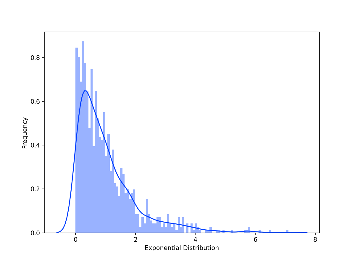
The distribution has a peak between 0 and 1, and a sharp exponential decrease on the right. Next, we'll draw random samples from the exponential distribution. Each sample will be of size=1000 having the same "width" or scale. Next, we'll draw three different sets of samples (n=25, n=50, n=1000) to see how the increase in sample number approximates the normal distribution better. Finally, we are going to demonstrate the Central Limit Theorem graphically.
# Create a list of means for each set of samples

###
# Initialize the list to hold the means
rs_means_n25 = []
# Loop 25 times, fill the list with 25 sample means
for i in range(25):
    # Draw random samples from the exponential distribution
    rs_exp = np.random.exponential(scale=1.0, size=1000)
    # Append the mean of the random sample
    rs_means_n25.append(rs_exp.mean())

###
# Initialize the list to hold the means
rs_means_n100 = []

# Loop 100 times, fill the list with 100 sample means
for i in range(100):
    # Draw random samples from the exponential distribution
    rs_exp = np.random.exponential(scale=1.0, size=1000)
    # Append the mean of the random sample
    rs_means_n100.append(rs_exp.mean())

###
# Initialize the list to hold the means
rs_means_n1000 = []
# Loop 1000 times, fill the list with 1000 sample means
for i in range(1000):
    # Draw random samples from the exponential distribution
    rs_exp = np.random.exponential(scale=1.0, size=1000)
    # Append the mean of the random sample
    rs_means_n1000.append(rs_exp.mean())
# Create the figure, axes objects
fig, (ax1, ax2, ax3) = plt.subplots(1, 3, figsize=(10,4))
# Plot each example on the correspond axis
sns.histplot(rs_means_n25, kde=True, bins=100, ax=ax1)
ax1.set(xlabel='n=25', ylabel='Frequency')
sns.histplot(rs_means_n100, kde=True, bins=100, ax=ax2)
ax2.set(xlabel='n=100')
sns.histplot(rs_means_n1000, kde=True, bins=100, ax=ax3)
ax3.set(xlabel='n=1000');
fig.clf() #comment/delete to plot<Figure size 720x288 with 0 Axes>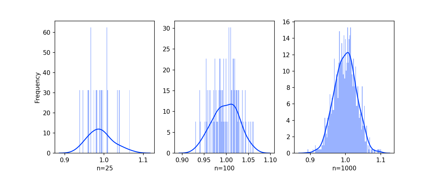
It's pretty cool to see the normal distribution take shape! As the number of samples draws from our original exponential distribution increases, the more normal the distribution becomes.
Challenge
We are using the applet linked here, we can experiment with drawing a different number of samples from three other distributions (exponential, uniform, and normal). Set the sample size=1 to see what the distribution looks like before we draw more than one sample. Increase the sample size by five each time and draw the samples again. Note when the resulting sampling distribution begins to approximate a normal distribution.
Additional Resources
Objective 07 - Explain the Purpose of and Identify Applications for Confidence Intervals
Overview
We've taken a closer look at standard error and what it means in terms of sampling from a population. We use this standard error in our hypothesis testing equations, but it has some implications for determining the actual significance of our result.
In this next objective (and the rest of the module), we will introduce the concept of confidence intervals, when to use them, and how to calculate them. But, first, let's review what we know about hypothesis testing and why we sometimes need different answers.
Hypothesis Testing Limits
First, consider how we have been testing our results so far. First, consider how we can test our results. We have performed t-tests until now, and will look into chi-square tests later on, to determine the significance of our results. But these tests have limited us to answering yes-or-no questions or rejecting (or not) a null hypothesis. We often want to know more about our results, such as how significant an observed effect is or how confident we are in our conclusions.
Another limitation with statistical testing is how influential the sample size is on the tests: the larger the sample, the smaller the error. When we look at how this "small" error propagates through, we can see the problem: the z-scores and t-scores become larger (because we're diving by a smaller denominator). As a result, small differences between a sample statistic and a population parameter seeming to be more significant than it is. So, larger sample size -> smaller standard error -> larger z-score/t-score -> deceptively significant value.
Well, what do we do? At this point, confidence intervals comes into play.
Confidence Intervals
When we want to know the significance of our result(s), we can calculate the confidence interval for that result. A confidence interval for a parameter is an interval computed from sample data by a method with a given probability C of producing an interval containing the true value of the parameter.
Let's unpack that definition a bit more. The confidence level C is a percent, and the values often used are 90%, 95%, and sometimes 99%. The interval is the estimated parameter plus or minus (+/-) the margin of error.
For example, if we chose a confidence level of 95% and drew a sample from our population, our result would fall within the confidence interval 95% of the time. However, if we wanted even more certainty, we might set the level at 99%: our result would be within the confidence interval 99% of the time.
Follow Along
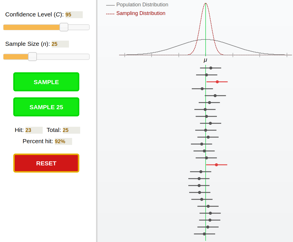
Let's look at confidence intervals graphically. We generated the following plot with this program: Statistical Applet: Confidence Intervals.
At the top, we can see an example population (solid gray line) and a sample (red dotted line). On the lower half of the graphic are lines with a dot in the middle. The dot is the sample mean, and the line through the dot is the confidence interval. For a confidence level set at 95%, the interval will cover the population mean. We can see in this particular example that the interval did not include the population mean in two cases (red lines).
Challenge
Using the same applet that we used to generate the above graphic, try adjusting the confidence interval and notice what happens to the size of the lines. In addition, change the sample size and observe how that affects the percent of samples that have intervals covering the population mean (the "percent hit" in the applet)
Additional Resources
Guided Project
Open DS_121_ttests_confidence_intervals.ipynb in the GitHub repository below to follow along with the guided project:
Guided Project Video
Module Assignment
Complete the Module 1 assignment to practice hypothesis testing and confidence intervals you've learned. The assignment covers formulating hypotheses, performing t-tests, calculating p-values, and interpreting statistical significance.