Module 3: Bayesian Statistics
Module Overview
In this module, we'll explore an alternative approach to statistics: the Bayesian perspective. Unlike the frequentist approach we've been using so far, Bayesian statistics treats probability as a measure of belief that can be updated as new evidence emerges.
So far, all statistics we've studied are frequentist statistics - drawing conclusions about an entire population or process by generalizing from the frequency or proportion of observed data. Frequentist statistics is well established and is still the default in most situations - but Bayesian statistics is an increasingly popular approach and an arguably better model for our brains and how we form and update beliefs based on evidence.
Learning Objectives
- Understand conditional probability
- Compare and contrast Frequentists and Bayesian philosophical approaches
Objective 01 - Understand Conditional Probability Notation and Be Able to Apply Them
Overview
We're going to change gears in this module and look at a different way of thinking about probability and inferential statistics, called Bayesian statistics. But before we can dive into the Bayesian world, we need to review some additional concepts in probability, specifically conditional probability.
Conditional Probability
First, let's review some mathematical notations for probabilities that will be useful for the rest of this module.
To illustrate the examples, we will use a deck of cards.
A deck of cards has 52 cards: 13 cards each of four different symbols (clubs, spades, hearts, diamonds), two colors (black - clubs, spades, and red - hearts, diamonds), and four of each number/“face” (Ace-10 and Jack, Queen, and King).
Let's list a few examples so we can see how probabilities are written (assume we start with a complete deck each time):
- randomly drawing a red card is 26/52; P(red card) = 26/52 (or 13/26)
- randomly drawing a heart is 13/52; P(hearts) = 13/52
- randomly drawing a Queen is 4/52; P(Queen) = 4/52 (or 1/13)
- randomly drawing a 7 of diamonds is 1/52; P(7 diamonds) = 1/52
Now, let's look at the probability when a card is drawn and not replaced. First, the probability of randomly drawing a red card is P(red card) = 26/52. If you draw a red card, there are now only 25 red cards left in the deck. So the probability of drawing a red card again is 25/51. This second probability is conditional on a red card being drawn first and not replaced. We could write this more formally as:
- Event A = red card and Event B = red card
- P(A) is the probability of drawing a red card from a complete deck P(A) = 26/52
- P(B|A) is read as the “Probability of B given A” and is equal to P(B|A) = 25/51
The total probability of drawing two red cards is P(A and B) = P(A) * P(B|A).
This is equal to P(A and B) = (26/52) * (25/51) = 25/102 or about 24.5%
Rearrange
We can use algebraic properties to rearrange the terms on each side of the equation.
- Start with: P(A and B) = P(A) * P(B|A)
- Switch sides: P(A) * P(B|A) = P(A and B)
- Divide each side by P(A): P(B|A) = P(A and B) / P(A)
Now we have an equation that reads, “The probability of B given A is equal to the probability of A and B divided by the probability of A."
Let's work through a few more examples in the next section before moving onto the suggested challenge.
Follow Along
Consider the following set-up, where we have a collection of marbles with the colors and quantities specified in the table:
Marble Data
| size | color | amber | bronze | cobalt |
|---|---|---|---|---|
| small | 7 | 2 | 6 | 15 |
| medium | 8 | 4 | 3 | 15 |
| large | 2 | 4 | 7 | 13 |
| total | 17 | 10 | 16 | 43 |
- What is the probability that we'll draw a medium cobalt marble?
P(M) = 3/43 - What is the probability we'll draw a large bronze marble?
P(large-bronze) = 4/43 - What is the probability we'll draw a small marble after drawing a large marble?
P(L and S) = P(L) * P(S|L)
P(L and S) = 13/43 * 15/42 = 65/602 (about 11%) - What is the probability of drawing a small cobalt marble and then a large cobalt marble?
P(SC and LC) = P(SC) * P(LC|SC)
P(SC and LC) = 6/43 * 7/42 = 1/43 (about 2%) - What is the probability of drawing two medium amber marbles?
P(MA and MA) = P(MA) * P(MA|MA)
P(MA and MA) = 8/43 * 7/42 = 4/129 (about 3%)
Challenge
Using the table above, try out some other combinations of marble selections and calculate the probabilities.
Additional Resources
Objective 02 - Compare and Contrast Frequentist and Bayesian Approaches to Inference
Overview
In the first objective, we hinted at the two different ways of thinking about probability and statistics. These two approaches are called “frequentist” and “Bayesian.” So far in this unit, we have been viewing probabilities (and the statistics calculated from them) from the frequentist side of things. Let's review our interpretations so far and then look in more detail at how the Bayesian interpretation is different.
Frequentist Interpretation
Our examples so far have focused on the probabilities of dice rolls and coin tosses, and the statistical significance of the different results. From the frequentist perspective, only these types of events (repeatable and random) can have probabilities determined by looking at many events over time. But this interpretation doesn't cover all needs or uses in statistics; there are cases where having a “belief” in the occurrence of some event is applicable. This belief is called a prior belief and is part of the basis for the Bayesian interpretation of probability.
Bayesian Interpretation
A Bayesian approach uses previous results to assign a probability to events like the outcome of a presidential election, which is something that isn't repeatable thousands of times. This type of prediction involves using prior information, data, or other information to inform the current prediction. For example, various fields of experimental research use Bayesian statistics to make predictions based on their prior experimental results. These are two example situations where we don't have a way to repeatedly repeat the experiment to determine the probability of the event or result occurring.
Conditional Probabilities
We looked at conditional probabilities in the last objective, where calculating the likelihood of some event depends on the probability of a different event having occurred. Next, we will formally write out the Bayes' Theorem with our new understanding of using prior knowledge, also called “priors.”
Follow Along
Using the probabilities of two events E1 and E2, Bayes' Theorem can be stated as:
P(E1 | E2) = P(E2 | E1) * P(E1) / P(E2)where:
- P(E1): Prior probability
- P(E2): Evidence
- P(E2 | E1): Likelihood
- P(E1 | E2): Posterior probability
Prior probability
The prior probability of an event is its probability obtained from some information known beforehand. But what does “before” or prior mean? We can think of this value as the probability of the event, given the information that's already known. Let's use an example where we would like to determine the probability of the weather being sunny. The prior probability would be the knowledge of how many times it has been sunny on this particular calendar date.
Evidence
We can use current evidence to update our prediction. For example, the evidence for our sunny weather example could be the probability of the atmospheric pressure being high - P(High Pressure). This equation is the probability of having high pressure, whether it's cloudy or sunny.
Likelihood
The likelihood represents a conditional probability, where the occurrence of one event depends on the other event having also occurred. In the weather example, this is the probability of having high pressure with it also being sunny.
Posterior probability
The term on the left is the posterior probability (or “after” probability) or also just the “posterior.” It represents the updated prior probability after taking into account some new piece of information.
Putting all these terms together, the equation would look like this:
P(Sunny | High Pressure) = P(High Pressure | Sunny) * P(Sunny) / P(High Pressure)Calculate the probability
We can assign probabilities to each of the above quantities and then calculate the posterior probability. For example, let's assume the probability of sunny weather is P(Sunny) = 0.5; the probability of high pressure is P(High Pressure) = 0.7; and the probability of high pressure if it's sunny is P(High Pressure | Sunny) = 0.9.
P(Sunny | High Pressure) = (0.9 * 0.5) / 0.7 = 0.64 which is a 64% percent probability that
it will be sunny if there is also high pressure.
Challenge
Set up your Bayesian situation and identify the prior probability, evidence, likelihood, and posterior probability. It would be helpful to write it out, as we have shown in the example above.
Additional Resources
Objective 03 - Use Bayes' Theorem to Update a Prior Probability Iteratively (Remove)
Overview
We've now seen Bayes' Theorem and how to write it out with mathematical notation. And we've done a lot of coding to compute t-tests, chi-square tests, and p-values. So, now it's time to put Bayes' theorem into practice and use it to update a prior probability.
Follow Along
We'll use an example of the probability of getting heads or tails on a coin toss. The example code comes from this website, and can also be downloaded there to experiment with on your computer.
This example code includes a way to create a biased coin that prefers one side over the other. Our job is to demonstrate that we can determine the bias by flipping the coin and updating after each flip.
# The example code is from this website:
# https://www.probabilisticworld.com/calculating-coin-bias-bayes-theorem/

# Import the usual libraries
import numpy as np
import matplotlib.pyplot as plt

# Set the number of flips
N = 15000

# Set the bias of the coin
BIAS_HEADS = 0.6

# The range of biases the coin could have
# (0, 0.01, 0.02, ... 0.98, 0.99, 1)
bias_range = np.linspace(0, 1, 101)

# Uniform prior distribution
# (start with coins that have the same bias)
prior_bias_heads = np.ones(len(bias_range)) / len(bias_range)

# Create a random series of 0's and 1's (coin flips) with the bias
flip_series = (np.random.rand(N) <= BIAS_HEADS).astype(int)

# For each flip, calculate the probabilities and update
for flip in flip_series:
    likelihood = bias_range**flip * (1-bias_range)**(1-flip)
    evidence = np.sum(likelihood * prior_bias_heads)
    prior_bias_heads = likelihood * prior_bias_heads / evidence

# Create the plot
plt.figure(figsize=(8,6))
plt.plot(bias_range, prior_bias_heads)
plt.xlabel('Heads Bias')
plt.ylabel('P(Heads Bias)')

plt.clf() #comment/delete to show plot
<Figure size 576x432 with 0 Axes>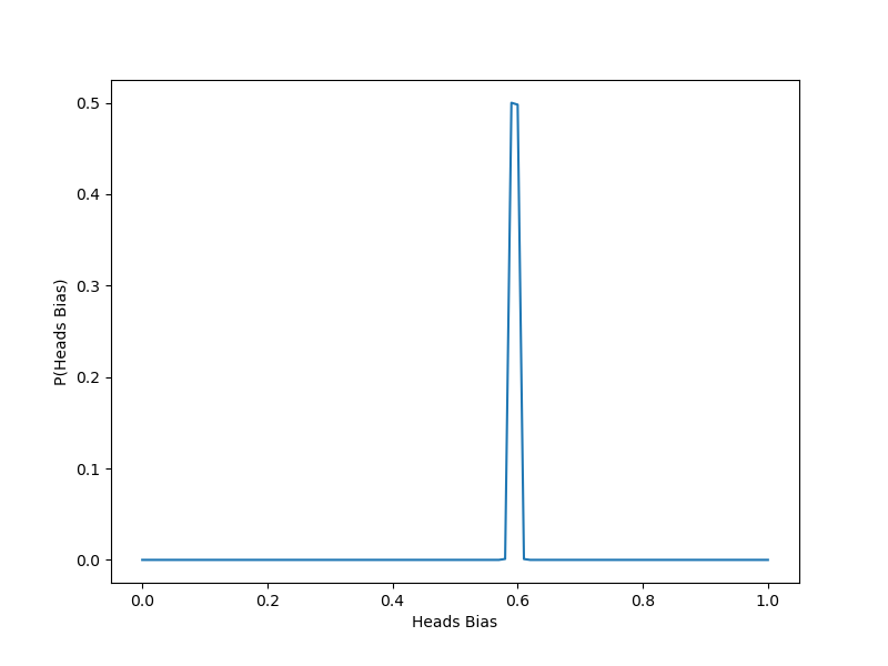
We can see that the bias is estimated correctly! First, we set the bias as 0.6 and generated coins with this bias. Then by going through each flip in the series of biased flips, we updated the probabilities, eventually resulting in the predictions confirming the bias.
Challenge
Using the above code, try changing a few of the parameters and seeing how your bias probability changes:
- Set the number of flips to a lower number and see if the result is still accurate
- Change the bias and see that it correctly predicts the new value
- Experiment to see if changing the bias and number of flips together has any affect on the results
Additional Resources
Guided Project
Open DS_123_Bayesian_Inference.ipynb in the GitHub repository below to follow along with the guided project:
Guided Project Video
Module Assignment
Complete the Module 3 assignment to practice Bayesian statistics techniques you've learned.
Assignment Solution Video
Resources
Bayesian Statistics Resources
- An Intuitive Explanation of Bayes' Theorem
- Bayesian Statistics for Beginners
- Seeing Theory: Bayesian Inference