Module 2: Random Forests
Module Overview
In this module, you will learn about Random Forests, a powerful ensemble learning technique that builds upon the foundation of decision trees. Random Forests combine multiple decision trees to create a more robust, accurate, and stable model that mitigates many of the limitations of individual decision trees.
You'll learn how Random Forests work, their advantages over single decision trees, and how to implement and tune them effectively using scikit-learn. This module will also introduce you to the concept of ensemble learning and its benefits in machine learning.
Learning Objectives
- Understand how categorical encoding effects tree based models differently
- Ordinal Encoding of High Cardinality Categoricals
- Understand how tree based ensembles reduce overfitting
- Build & Interpret Random Forests using scikit learn
Objective 01 - use scikit-learn for random forests
Overview
We've covered some advantages of using decision trees over other types of models, including how easy they are to to implement and interpret. One disadvantage however, with a decision tree is that they tend to overfit or model the training data too closely. Because of this, they don't generalize well to new data.
To solve the problem of overfitting we can use the results returned from more than one decision tree. A random forest is an ensemble method where many decision trees are trained. Combining the results of two (or more) decision trees improves the fit. We train a decision tree on a random subset of the data, combine the results with other randomly-trained trees, and thus have a random forest.
Random Forest
We've already trained a decision tree on the wine quality data set. It's time for a random forest to see
if we can improve on the accuracy. The RandomForestClassifier is implemented in almost the
same way as the DecisionTreeClassifier.
Follow Along
The wine data set is available in the scikit-learn datasets library.
# Import libraries and data sets
from sklearn.datasets import load_wine
import pandas as pd

# Load the data and convert to a DataFrame
data = load_wine()
df_wine = pd.DataFrame(data.data, columns=data.feature_names)
df_wine['target'] = pd.Series(data.target)
df_wine.head()| alcohol | malic_acid | ash | alcalinity_of_ash | magnesium | total_phenols | flavanoids | nonflavanoid_phenols | proanthocyanins | color_intensity | hue | od280/od315_of_diluted_wines | proline | target | |
|---|---|---|---|---|---|---|---|---|---|---|---|---|---|---|
| 0 | 14.23 | 1.71 | 2.43 | 15.6 | 127.0 | 2.80 | 3.06 | 0.28 | 2.29 | 5.64 | 1.04 | 3.92 | 1065.0 | 0 |
| 1 | 13.20 | 1.78 | 2.14 | 11.2 | 100.0 | 2.65 | 2.76 | 0.26 | 1.28 | 4.38 | 1.05 | 3.40 | 1050.0 | 0 |
| 2 | 13.16 | 2.36 | 2.67 | 18.6 | 101.0 | 2.80 | 3.24 | 0.30 | 2.81 | 5.68 | 1.03 | 3.17 | 1185.0 | 0 |
| 3 | 14.37 | 1.95 | 2.50 | 16.8 | 113.0 | 3.85 | 3.49 | 0.24 | 2.18 | 7.80 | 0.86 | 3.45 | 1480.0 | 0 |
| 4 | 13.24 | 2.59 | 2.87 | 21.0 | 118.0 | 2.80 | 2.69 | 0.39 | 1.82 | 4.32 | 1.04 | 2.93 | 735.0 | 0 |
# Separate into features and target

X = df_wine.drop('target', axis=1)
y = df_wine['target']

# Import train_test_split function
from sklearn.model_selection import train_test_split

# Split dataset into training set and test set
X_train, X_test, y_train, y_test = train_test_split(X, y, test_size=0.25)
#Import Random Forest Model
from sklearn.ensemble import RandomForestClassifier
#Create a Gaussian Classifier
rf_classifier=RandomForestClassifier(n_estimators=100)
#Train the model using the training sets y_pred=clf.predict(X_test)
rf_classifier.fit(X_train,y_train)
y_pred=rf_classifier.predict(X_test)
# Fit the model with our logistic regression classifier
print("model score: %.3f" % rf_classifier.score(X_test, y_test))
model score: 0.978Now we can compare this to the results of the decision tree model we fit in the previous objective.
# Use the decision tree classifier
from sklearn.tree import DecisionTreeClassifier

# Instantiate the classifier
dt_classifier=DecisionTreeClassifier()

# Train the model using the training sets
dt_classifier.fit(X_train,y_train)

# Find the model score
print("Decision tree model score: %.3f" % dt_classifier.score(X_test, y_test))
Decision tree model score: 0.911The decision tree model didn't perform as well as the random forest model, which was expected. Let's compare the feature importance for the models side-by-side.
# Plot the feature importances
import matplotlib.pyplot as plt

rf_importances = pd.Series(rf_classifier.feature_importances_, X.columns)
dt_importances = pd.Series(dt_classifier.feature_importances_, X.columns)

# Plot top n feature importances
n = 13
fig, (ax1, ax2) = plt.subplots(1,2,figsize=(12,n/2))
ax1.set_title(f'Decision Tree: Top {n} features')
ax2.set_title(f'Random Forest: Top {n} features')
dt_importances.sort_values()[-n:].plot.barh(ax=ax1)
rf_importances.sort_values()[-n:].plot.barh(ax=ax2)

fig.show()
<Figure size 864x468 with 0 Axes>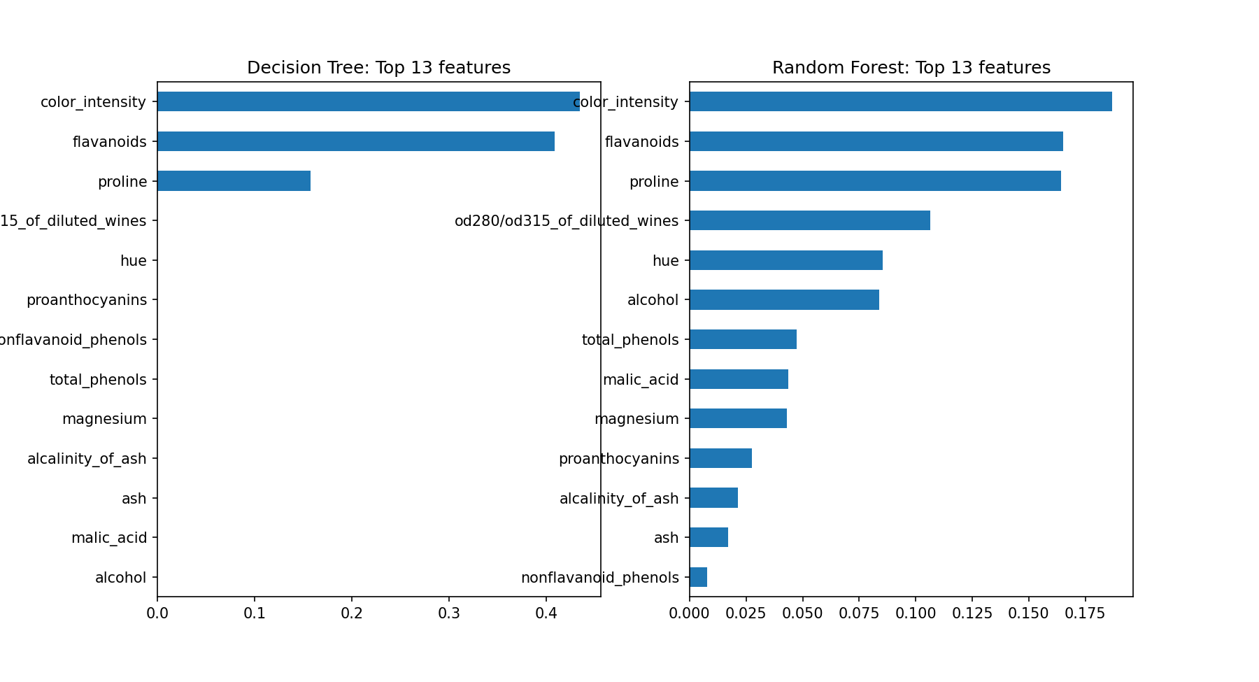
Challenge
As with the challenge in the previous objective, try using different parameters in the
RandomForestClassifier and observing how the model results change. Some parameters to
adjust are the max_depth and the num_estimators. Are the feature importances
different?
Additional Resources
Objective 02 - implement ordinal encoding with high-cardinality categoricals
Overview
In a previous module we looked at one-hot encoding, where we created separate columns for each class represented in the data. Each column is a series of '0' and '1' to indicate if that class is represented in the given row. If we had numerous classes in one of the feature columns, the size of the resulting one-hot encoded DataFrame would grow very large. For example, if we had a column with 100 different classes, we would need an additional 100 columns to represent the one-hot encoding.
Data with a large number of classes is said to have high cardinality. One solution to use for data with high cardinality is to ordinal encode the classes. This would assume that the values in the data have some relationship to each other, as they are being "ordered". For our example here we'll assume the values are not related.
Follow Along
To make this example easier to follow, we'll generate some data and use both the label encoder and the ordinal encoder.
# Imports
import numpy as np
import pandas as pd

# Create the DataFrame
df = pd.DataFrame({
    'color':["a", "c", "a", "a", "b", "b", "d", "d", "c"],
    'outcome':[1, 2, 0, 0, 1, 1, 3, 3, 2]})

# set up X and y
X = df.drop('outcome', axis = 1)
y = df.drop('color', axis = 1)
# Label encoding
from sklearn.preprocessing import LabelEncoder
label_enc = LabelEncoder()
encoded = label_enc.fit_transform(np.ravel(X))
print("\n The result of transforming X with LabelEncoder:")
print(encoded)
print(type(encoded))The result of transforming X with LabelEncoder:
[0 2 0 0 1 1 3 3 2]
<class 'numpy.ndarray'># Ordinal encoding
from sklearn.preprocessing import OrdinalEncoder
ordinal_enc = OrdinalEncoder()
ordinal_enc.fit_transform(X, y['outcome'])array([[0.],
[2.],
[0.],
[0.],
[1.],
[1.],
[3.],
[3.],
[2.]])
Challenge
Try creating your own data set to practice some encoding!
Additional Resources
Objective 03 - understand how categorical encodings affect trees differently compared to linear models
Overview
When a decision tree model is fit, the algorithm needs to decide how to make the split. When the tree is splitting on categorical values, it has to consider all possible pair subsets. If there are a lot of classes in the categorical variables, this splitting decision becomes more complicated and computationally intensive.
If we use one-hot encoding on our categorical variables, we can also introduce another problem with the sparse matrices that result from the encoding. If the data contains both continuous numeric features and one-hot encoded categorical features, then the continuous variables will be assigned higher feature importance because splitting on them will reduce the variance or impurity more than the categorical variables.
Follow Along
To explore how categorical encodings affect different types of models, we're going to work with a dataset that has a number of categorical features. The mushroom dataset is available from the UCI Machine Learning website.
This dataset includes descriptions of 23 species of gilled mushrooms found in North America. From the properties of each type of mushroom we are trying to predict which class it belongs to: definitely edible or definitely poisonous. Let's load in the data and get started.
# Imports
import pandas as pd
import numpy as np

# Load the data (saved on GitHub)
url = 'https://tinyurl.com/y884c98f'
mushrooms = pd.read_csv(url)
mushrooms.head()| class | cap-shape | cap-surface | cap-color | bruises | odor | gill-attachment | gill-spacing | gill-size | gill-color | ... | stalk-surface-below-ring | stalk-color-above-ring | stalk-color-below-ring | veil-type | veil-color | ring-number | ring-type | spore-print-color | population | habitat | |
|---|---|---|---|---|---|---|---|---|---|---|---|---|---|---|---|---|---|---|---|---|---|
| 0 | p | x | s | n | t | p | f | c | n | k | ... | s | w | w | p | w | o | p | k | s | u |
| 1 | e | x | s | y | t | a | f | c | b | k | ... | s | w | w | p | w | o | p | n | n | g |
| 2 | e | b | s | w | t | l | f | c | b | n | ... | s | w | w | p | w | o | p | n | n | m |
| 3 | p | x | y | w | t | p | f | c | n | n | ... | s | w | w | p | w | o | p | k | s | u |
| 4 | e | x | s | g | f | n | f | w | b | k | ... | s | w | w | p | w | o | e | n | a | g |
5 rows × 23 columns
As we can see, most of the variables in this data set are categorical. We'll need to encode them to use in the models. To compare how different types of models handle encoded categorical variables, we'll use both a logistic regression and a tree-based model.
# Create the feature matrix (drop the target column)
X = mushrooms.drop('class', axis=1)

# Create and encode the target column
from sklearn import preprocessing
le = preprocessing.LabelEncoder()
y = le.fit_transform(mushrooms['class'])
# Imports
from sklearn.compose import ColumnTransformer
from sklearn.pipeline import Pipeline
from sklearn.preprocessing import OneHotEncoder
# Use the decision tree classifier
from sklearn.tree import DecisionTreeClassifier
from sklearn.model_selection import train_test_split
# Set-up the one-hot encoder
categorical_features = X.columns
categorical_transformer = Pipeline(steps=[('onehot', OneHotEncoder())])
# Set up our preprocessor/column transformer
preprocessor = ColumnTransformer(
transformers=[
('cat', categorical_transformer, categorical_features)])
# Add the classifier to the preprocessing pipeline
pipeline = Pipeline(steps=[('preprocessor', preprocessor),
('classifier', DecisionTreeClassifier())])# Apply the pipeline
# Separate into training and testing sets
X_train, X_test, y_train, y_test = train_test_split(X, y, test_size=0.25)
# Fit the model with our decision tree classifier
pipeline.fit(X_train, y_train)
print("Decision tree model score: %.3f" % pipeline.score(X_test, y_test))Decision tree model score: 1.000# Use the logistic regression classifier
from sklearn.linear_model import LogisticRegression
# Add the classifier to the preprocessing pipeline
pipeline_logreg = Pipeline(steps=[('preprocessor', preprocessor),
('classifier', LogisticRegression())])
# Apply the pipeline
# Separate into training and testing sets
X_train, X_test, y_train, y_test = train_test_split(X, y, test_size=0.25)
# Fit the model with our logistic regression classifier
pipeline_logreg.fit(X_train, y_train)
print("Logistic regression model score: %.3f" % pipeline_logreg.score(X_test, y_test))Logistic regression model score: 1.000# Set-up the ordinal encoder
from sklearn.preprocessing import OrdinalEncoder
categorical_features = X.columns
categorical_transformer = Pipeline(steps=[('ordinal', OrdinalEncoder())])
# Set up our preprocessor/column transformer
preprocessor_ord = ColumnTransformer(
transformers=[
('cat', categorical_transformer, categorical_features)])
# Add the classifier to the preprocessing pipeline
pipeline_ord = Pipeline(steps=[('preprocessor_ord', preprocessor_ord),
('classifier', DecisionTreeClassifier())])# Fit the model with our decision tree classifier
pipeline_ord.fit(X_train, y_train)
print("Decision tree model score (ordinal encoded): %.3f" % pipeline_ord.score(X_test, y_test))Decision tree model score (ordinal encoded): 1.000Additional Resources
Objective 04 - understand how tree ensembles reduce overfitting compared to a single decision tree with unlimited depth
Overview
In the first objective of this module we discussed how decision trees can tend to overfit on the training data. Ensemble methods like the random forest help to reduce this by averaging results from numerous models. Now we'll look more closely at the accuracy of both the decision tree model and random forest model for different depths.
We'll be visiting the penguins data set again and predict the class (sex) that each penguin belongs to. Lets compare the predictions of tree-based models with that of a logistic regression model. We will use both the RandomForestClassifier and the DecisionTreeClassifier, and plot the accuracy against the depth of the tree.
Follow Along
# Import libraries and load in the data
import pandas as pd
import seaborn as sns

penguins = sns.load_dataset("penguins")

# Remove NaNs and nulls
penguins.dropna(inplace=True)

display(penguins.head())
species island bill_length_mm bill_depth_mm flipper_length_mm body_mass_g sex
0 Adelie Torgersen 39.1 18.7 181.0 3750.0 Male
1 Adelie Torgersen 39.5 17.4 186.0 3800.0 Female
2 Adelie Torgersen 40.3 18.0 195.0 3250.0 Female
4 Adelie Torgersen 36.7 19.3 193.0 3450.0 Female
5 Adelie Torgersen 39.3 20.6 190.0 3650.0 MaleLet's use only the numeric columns to predict the class (male or female). We'll use a logistic regression, decision tree, and random forest.
# Create feature matrix
X = penguins.drop(['species', 'island', 'sex'], axis=1)

# Create the target array
from sklearn import preprocessing
le = preprocessing.LabelEncoder()
y = le.fit_transform(penguins['sex'])

# Create training and testing data
from sklearn.model_selection import train_test_split
X_train, X_test, y_train, y_test = train_test_split(X, y, test_size=0.25)
# Import the classifiers

from sklearn.linear_model import LogisticRegression
from sklearn.tree import DecisionTreeClassifier
from sklearn.ensemble import RandomForestClassifier
# Fit the model with a logistic regression classifier

logreg = LogisticRegression()
logreg.fit(X_train, y_train)
print("Logistic regression model score: %.3f" % logreg.score(X_test, y_test))
Logistic regression model score: 0.798# Fit the model with a decision tree classifier
tree = DecisionTreeClassifier()
tree.fit(X_train, y_train)
print("Decision tree model score: %.3f" % tree.score(X_test, y_test))Decision tree model score: 0.821# Fit the model with a random forest classifier
trees_rand = RandomForestClassifier()
trees_rand.fit(X_train, y_train)
print("Random forest model score: %.3f" % trees_rand.score(X_test, y_test))Random forest model score: 0.893Look at accuracy for a different number of trees
# Fit the model with a decision tree classifier

tree = DecisionTreeClassifier(max_depth=100)
tree.fit(X_train, y_train)
print("Decision tree model score: %.3f" % tree.score(X_test, y_test))

print("Decision tree model score: %.3f" % tree.score(X_train, y_train))
Decision tree model score: 0.821
Decision tree model score: 1.000Look at training accuracy vs. test accuracy
# Decision tree
accuracy_train = []
accuracy_test = []

for i in range(1, 160, 5):
    tree = DecisionTreeClassifier(max_depth=i)
    tree.fit(X_train, y_train)
    accuracy_test.append(tree.score(X_test, y_test))
    accuracy_train.append(tree.score(X_train, y_train))
# Look at training accuracy vs. test accuracy
# Random forest
rf_accuracy_train = []
rf_accuracy_test = []
for i in range(1, 160, 5):
tree = RandomForestClassifier(max_depth=i)
tree.fit(X_train, y_train)
rf_accuracy_test.append(tree.score(X_test, y_test))
rf_accuracy_train.append(tree.score(X_train, y_train))Plot the results of the train vs. test accuracy
import matplotlib.pyplot as plt

fig, (ax1, ax2) = plt.subplots(1,2, figsize=(10,5))

xvals = range(1, 160, 5)
ax1.plot(xvals, accuracy_train, color='b', label='train')
ax1.plot(xvals, accuracy_test, color='red', label='test')
ax1.legend()

ax2.plot(xvals, rf_accuracy_train, color='b', label='train')
ax2.plot(xvals, rf_accuracy_test, color='red', label='test')
ax2.legend()

ax1.set_ylim([0.65, 1.02])
ax2.set_ylim([0.65, 1.02])

ax1.set_xlabel('Number of nodes (max depth of the tree)')
ax2.set_xlabel('Number of nodes (max depth of the tree)')
ax1.set_ylabel('Accuracy')
ax1.set_title('Decision Tree')
ax2.set_title('Random Forest')

fig.show()
<Figure size 720x360 with 0 Axes>
mod2_obj4_accuracy.pngChallenge
In this challenge, look at how the training and testing accuracy changes by setting the number of trees used in the random forest classifier (the n_estimators parameter). If n_estimators=1 then you would have a single decision tree classifier. The accuracy should increase with increasing trees.
Additional Resources
Guided Project
Open JDS_SHR_222_guided_project_notes.ipynb in the GitHub repository below to follow along with the guided project:
Guided Project Video
Module Assignment
Complete the Module 2 assignment to practice Random Forest techniques you've learned.
It's time to apply what you've learned about Random Forests to improve your predictions in the Kaggle competition!