Module 2: Exploratory Data Analysis & Feature Engineering
Module Overview
In this module, you'll learn how to work with data using Google Colab and Pandas. You'll discover how to read and load datasets, explore your data using Pandas' powerful analysis tools, perform feature engineering to transform your data, and master string functions in Pandas for text data manipulation.
Learning Objectives
- Read and load datasets using Google Colab and Pandas
- Explore and analyze data using Pandas' functionality
- Apply feature engineering techniques to transform and prepare data
- Master string functions in Pandas for text data manipulation
Detailed Objective: Exploratory Data Analysis (EDA)
Exploratory data analysis (EDA) is an essential part of learning to be a data scientist. And something that experienced data scientists do regularly.
We'll be using some of the numerous tools available in the pandas library. Earlier in the module, we learned how to load datasets into notebooks. So now that we have all this data, what do we do with it?
Basic Information Methods
We can use a few methods to quickly look at your DataFrame and get an idea of what's inside. Here are some of the most common descriptions of what each method does:
| Method | Description |
|---|---|
df.shape |
Display the size (rows, columns) |
df.head() |
Display the first 5 rows (we can display first n rows by including the number in parenthesis) |
df.tail() |
Display the last 5 rows (we can display last n rows by including the number in parenthesis) |
df.describe() |
Display the statistics of numerical data types |
df.info() |
Display the number of entries (rows), number of columns, and the data types |
Column-specific Methods
Sometimes we don't want to look at the entire DataFrame and instead focus on a single column or a few
columns. There are a few ways to select a column, but we'll mainly use the column name. For example, if
we have a DataFrame called df and a column named "column_1," we could select just a single
column by using df["column_1"]. Once we have a single column chosen, we can use some of the
following methods to get more information.
| Method | Description |
|---|---|
df.columns |
Print a list of the columns |
df['column_name'] |
Select a single column (returns a Series) |
df['column_name'].value_counts() |
Count the number of object and boolean occurrences |
df.sort_values(by='column_name') |
Sort the values in the given column |
df.drop() |
Remove rows or columns by specifying the label or index of the row/column |
Handling Missing Values
With a lot of data comes the unavoidable fact that some of it will be messy. Messy data means that there will be missing values, "not-a-number" (NaN) occurrences, and problems with zeros not being zero. Fortunately, several pandas methods make dealing with the mess a little easier.
| Method | Description |
|---|---|
df.isnull().sum() |
Count and sum the number of null occurrences (NaN or None) |
df.fillna() |
Fill NaN values in a variety of ways |
df.dropna() |
Remove values that are NaN or None; by default removes all rows with NaNs |
Practical Example
Let's see a practical example of EDA using the M&Ms dataset, which is small and contains both numeric and object (string) data types:
# Import pandas
import pandas as pd

# Read the data from the website
url_mms = 'https://tinyurl.com/mms-statistics'
df = pd.read_csv(url_mms)

# Look at the shape
df.shape  # returns (816, 4)

# Look at the head of the file
df.head()
When we run df.head(), we'll see the first 5 rows of the dataset with columns 'type',
'color', 'diameter', and 'mass'. We can get more information about the dataset with:
# DataFrame information
df.info()
The output will tell us we have 816 entries, 4 columns, and reveal the data types. Let's also check the statistics of the numeric columns:
# DataFrame describe
df.describe()
This shows statistics like count, mean, standard deviation, min/max, and percentiles for numeric columns.
What if we want to count how many of each candy type we have?
Objective 01 - Load a CSV Dataset From a URL Using Pandas read_csv
Overview
We will be working with data in many different forms throughout this course. But before we can start to do anything with that data, we need to load it into our workspace. So we'll be working in Google Colab notebooks, focusing on loading data into that environment. Eventually, you'll be working with a local Jupyter environment, but these instructions will work for that, too.
Pandas
You are likely already familiar with the Python data analysis library pandas. We'll provide a quick overview here and then work through some examples in the next section.
The pandas library provides extensive data analysis and data manipulation tools. It also includes data structures (Series, DataFrames) that work well with various data types, including tabular data, time-series data, and arbitrary matrix data (for example, columns with different data types).
Reading files using
To start, we'll learn how to load data with one of the most common pandas methods:
read_csv. This method
reads data in the comma-separated value or CSV format: the values in each row are separated by a comma,
and new lines (rows) begin on the following line. A CSV file can be read from a locally saved file on
your computer or loaded from a URL. We'll practice both these techniques in this module, starting with
data that is stored online.
As with many pandas methods, there are several options to use with read_csv. To learn about
these, an
excellent place to begin is with some of the official documentation.
For this first exercise, we will use the default read_csv parameters. Time to read in some
data!
Follow Along
We will practice using the read_csv method to load a data set from a URL. The UCI Machine
Learning Repository has a great selection of data sets, and many are in a good format for
practicing.
The Tic-Tac-Toe Endgame data set is a manageable size (~900 rows) and has ten columns; this size makes it easy to examine once we read it in. To retrieve the URL, click on the above link and click on the Download: Data Folder link. You should see a list; right-click on tic-tac-toe data and select Copy link address.
In your notebook, you can use the following code to read in the data set:
# Import pandas with the standard alias
import pandas as pd

# Set a variable to the URL you copied above
url = 'https://archive.ics.uci.edu/ml/machine-learning-databases/tic-tac-toe/tic-tac-toe.data'

# Read or load the data
df = pd.read_csv(url)
Great! If you copied the link correctly, you should have sucessfully loaded the data set. A simple check is to type the variable name and run the cell:
# Look at the data (df)
df.head()
| x | x.1 | x.2 | x.3 | o | o.1 | x.4 | o.2 | o.3 | positive | |
|---|---|---|---|---|---|---|---|---|---|---|
| 0 | x | x | x | x | o | o | o | x | o | positive |
| 1 | x | x | x | x | o | o | o | o | x | positive |
| 2 | x | x | x | x | o | o | o | b | b | positive |
| 3 | x | x | x | x | o | o | b | o | b | positive |
| x | x | x | x | o | o | b | b | o | positive |
We can see that there isn't a header row (a row with labels for each column). To fix this, look up the information for this data set, and manually create a list of columns names; this list could be set as the header row.
Challenge
Since the data set we read above is missing a header row, this would be an excellent time to practice adding one. For the UCI Repository specifically, the information about the data sets is often located in the same “Data Folder” from where you downloaded it.
Here are some steps to get started:
- Navigate to the "Data Folder" and look for a file that ends in .names; view the file (download and open if needed) and learn what each column represents
- Create a Python list with column names; example:
mycols = ['col 1', 'col 2', 'col 3'](make sure the number of column names in your lists matches the number of columns in your data set) - Try this option first:
df = pd.read_csv(url, header=None) - And compare to this option:
df = pd.read_csv(url, header=1) - Using the column names you set above, try this option:
df = pd.read_csv(url, names=mycols)
Additional Resources
Objective 02- Load a CSV dataset from a local file using Pandas read_csv
Overview
When working with data sets, you'll find many of them conveniently stored online at various locations (UCI Repository, Kaggle, etc.). But you'll often want to download a data set to store it on your local computer. Storing the data set makes it easy to use tools on your computer to view and edit the file, in addition to having a copy stored on your hard drive.
The pandas read_csv() method can also read in locally saved files. Instead of providing the
URL, you will use the path to the file. Think of the path like the address of the file: it's a list of
directories leading to the file location. An example path might look like
/Users/myname/Documents/data_science/tic-tac-toe.data where the last part of the path is
the file name. To read in a local file with pandas, you can use the following code (assuming pandas has
been installed on your computer):
# Read in an example file (from a example user's Downloads folder)
import pandas as pd
df = pd.read_csv('/home/username/Downloads/tic-tac-toe.data')
Done! Common issues here are having an incorrect path listed for the file or an incorrect file name. You also need to make sure you include quotes (either single or double) around your path.
Since we are currently working in notebooks on Google Colab, we need to know how to get data loaded into that environment.
Google Colab
There are a few different ways to load files into your Colab notebook. The first one we will cover here
is loading a file from your computer. You need to have already downloaded and saved the file. The next
step is to use the files method from the google.colab package:
# Upload a file to Colab from your computer
from google.colab import files
uploaded = files.upload()
The system will prompt you to select a file.
Select the tic-tac-toe.data file you downloaded. It should be in your Downloads folder.
This should return a result that looks like this:
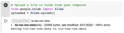
Now, we can read our file into a DataFrame:
# Store your uploaded file in a pandas DataFrame
df = pd.read_csv('tic-tac-toe.data')
Follow Along
Let's work through another example, where we read in a file from a notebook running locally and from a notebook running in Colab. We'll download another file from the UCI Machine Learning Repository: the Auto MPG Data Set.
Local Jupyter Notebook
If you are following along on your notebook running locally (on your computer, not on Google Colab), change the path to correspond to where you have saved the file on your computer.
# Load a file saved LOCALLY
import pandas as pd
df = pd.read_csv('/home/username/Downloads/auto-mpg.data')
Google Colab notebook
Now in a Colab notebook, we'll follow the same steps from the Overview and load this new data set and read it into a DataFrame:
from google.colab import files
uploaded = files.upload()

# A prompt will ask you to choose a file
# Choose a file

# Store your uploaded file in a pandas DataFrame
import io
df = pd.read_csv(io.BytesIO(uploaded['auto-mpg.data']))
In this case, we used the Python package io, which stands for input/output. The
io.BytesIO is reading data stored as bytes in an in-memory buffer (in this case in Colab).
You now have a new data set to explore!
Challenge
For more practice, look through the UCI Machine Learning Repository and find a data set to download to your computer. Make sure it is a CSV file and not in a different format. Upload into Google Colab and then load that file into a DataFrame.
Additional Resources
Objective 03 - Use Basic Pandas Functions for Exploratory Data Analysis-EDA Overview
Overview
Exploratory data analysis (EDA) is an essential part of learning to be a data scientist. And something that experienced data scientists do regularly.
We'll be using some of the numerous tools available in the pandas library. Earlier in the module, we learned how to load datasets into notebooks. So now that we have all this data, what do we do with it?
Basic Information
We can use a few methods to look at your DataFrame quickly and get an idea of what's inside. Here are some of the most common descriptions of what each method does:
| method | description |
|---|---|
df.shape |
display the size (x, y) |
df.head() |
display the first 5 rows ( we can display first n rows by including the number in parenthesis) |
df.tail() |
display the last 5 rows ( we can display last n rows by including the number in parenthesis) |
df.describe() |
display the statistics of numerical data types |
df.info() |
display the number of entries (rows), number of columns, and the data types |
Column-specific
Sometimes we don't want to look at the entire DataFrame and instead focus on a single column or a few
columns. There are a few ways to select a column, but we'll mainly use the column name. For example, if
we have a DataFrame called df and a column named “column_1,” we could select just a single
column by using df["column_1"]. Once we have a single column chosen, we can use some of the
following methods to get more information.
| method | description |
|---|---|
df.columns |
print a list of the columns |
df['column_name'] |
select a single column ( returns a Series) |
df['column_name'].value_counts() |
count the number of object and boolean occurrences |
df.sort_values(by='column_name') |
sort the values in the given column |
df.drop() |
remove rows or columns by specifying the label or index of the row/column |
Missing Values
With a lot of data comes the unavoidable fact that some of it will be messy. Messy data means that there will be missing values, “not-a-number” (NaN) occurrences, and problems with zeros not being zero. Fortunately, several pandas methods make dealing with the mess a little easier.
| method | description |
|---|---|
df.isnull().sum() |
count and sum the number of null occurrences (NaN or None) |
df.fillna() |
fill NaN values in a variety of ways |
df.dropna() |
remove values that are NaN or None; by default removes all rows with NaNs |
Follow Along
The above methods cover much ground, but we'll work through examples using them on a data set. But, first, we need some data. We'll use the M&Ms data set for this because it's small and contains both numeric and Object (string) data types.
# Import pandas
import pandas as pd

# Read the data from the website
url_mms = 'https://tinyurl.com/mms-statistics'
df = pd.read_csv(url_mms)

# Look at the shape
df.shape  # returns (816, 4)

# Look at the head of the file
df.head()| type | color | diameter | mass | |
|---|---|---|---|---|
| 0 | peanut butter | blue | 16.20 | 2.18 |
| 1 | peanut butter | brown | 16.50 | 2.01 |
| 2 | peanut butter | orange | 15.48 | 1.78 |
| 3 | peanut butter | brown | 16.32 | 1.98 |
| 4 | peanut butter | yellow | 15.59 | 1.62 |
Let's look at the information using df.info():
# DataFrame information
df.info()
<class 'pandas.core.frame.DataFrame'>
RangeIndex: 816 entries, 0 to 815
Data columns (total 4 columns):
type        816 non-null object
color       816 non-null object
diameter    816 non-null float64
mass        816 non-null float64
dtypes: float64(2), object(2)
memory usage: 25.6+ KB
From this, we can see the columns “type” and “color” are object data types, and “diameter” and “mass”
are numeric. We can use describe to print out the statistics for the numeric columns using
df.describe():
# DataFrame describe
df.describe()| diameter | mass | |
|---|---|---|
| count | 816.000000 | 816.000000 |
| mean | 14.171912 | 1.419632 |
| std | 1.220001 | 0.714765 |
| min | 11.230000 | 0.720000 |
| 25% | 13.220000 | 0.860000 |
| 50% | 13.600000 | 0.920000 |
| 75% | 15.300000 | 1.930000 |
| max | 17.880000 | 3.620000 |
DataFrame Columns
We can print out the columns of this data set with df.columns which returns an Index:
# DataFrame columns
df.columns
Index(['type', 'color', 'diameter', 'mass'], dtype='object')
To drop one of the columns, for example "mass", we'll use the df.drop() with the column
specified:
# Drop the mass column
df.drop(columns='mass').head()| type | color | diameter | |
|---|---|---|---|
| 0 | peanut butter | blue | 16.20 |
| 1 | peanut butter | brown | 16.50 |
| 2 | peanut butter | orange | 15.48 |
| 3 | peanut butter | brown | 16.32 |
| 4 | peanut butter | yellow | 15.59 |
We can also look at the number of different values in one of the columns. Let's see how many different values we have in the "type" column:
# Count the values in the 'type' column
df['type'].value_counts()
plain 462 peanut butter 201 peanut 153 Name: type, dtype: int64
We see an excellent display of how many plain, peanut butter, and peanut M&M types are present in the DataFrame.
Challenge
Now, while using the M&Ms data set, practice loading and exploring the DataFrame; specifically, learn if
there are any Null or NaN values in this data set and remove them if there are. You can also practice
using the df.sort_values() method on one of the numeric columns ('mass' or 'diameter')
Additional Resources
Objective 04 - Understand the Purpose of Feature Engineering
Overview
Why do we care about feature engineering?
When we begin working on a new project and a new data set, we have to consider how to make the best use of the information contained in the dataset. We want to get the most out of the data, without having to leave out useful information. It is also essential to ensure that the features we are using, are best suited for the type of modeling we would like to perform. In other words, what is the best representation of the data so that a model can learn from it? Choosing good features might allow you to use a less complex model, saving time on both implementation and interpretation.
Many of these considerations fall under the process of "feature engineering." So before we dig too deep, let's take a closer look at what features are.
What are features?
A feature is a measurable property or attribute, and is often something that is measured or observed. It can be a numeric feature (eg. temperature, weight, time etc.), or categorical (eg: sex, color, group, etc. ). We usually work with data in the form of a table, also called tabular data. The data is composed of rows (also called observations, instances or samples) and columns (also called variables or attributes). Some of the columns in a data set contain features, such as a column measuring the temperature of something over time (measurable observation). But other columns, like the index, would not be considered a feature.
Feature importance and selection
Not all features are equal when it comes to using them in creating a model. Depending on the problem you are solving, some features may be more beneficial than others. Therefore, some criteria can rank features, and then the analysis can only use the top-ranked feature.
Feature extraction
Feature extraction doesn't exactly sound like a process you would apply to data, but it's an integral part of feature engineering. The process can be complex, but it's taking high-dimensional data and reducing it without taking away any information.Some standard methods of feature extraction include Principal Component Analysis (PCA) and unsupervised clustering methods.
Feature construction
The process of feature construction is a little more straightforward compared to feature extraction. By combining, splitting apart, or otherwise modifying existing features, you can create new features.For example, when using data that consists of a calendar date, we could break the date variable into years, months, and days. A new feature could then be given as the year or the month by itself.
Feature engineering process
Here we describe a basic feature engineering process. We will cover the individual steps of the process in more detail as the course progresses.
- Brainstorming or testing features
- Deciding what features to create
- Creating features
- Checking how the features work with your model
- Improving your features if needed
- Go back to brainstorming/creating more features until the work is complete
Follow Along
Now that we know what features are and some methods used to select, extract, and construct features, we will use another practice data set to create some new features from the existing columns. Next, we'll use the M&Ms data set to make some new features from what already exists in the data set.
# Import our libraries
import pandas as pd

# Read in the M&Ms data into a DataFrame
mms = pd.read_csv('https://tinyurl.com/mms-statistics')

# Display the data
display(mms.head())| type | color | diameter | mass | |
|---|---|---|---|---|
| 0 | peanut butter | blue | 16.20 | 2.18 |
| 1 | peanut butter | brown | 16.50 | 2.01 |
| 2 | peanut butter | orange | 15.48 | 1.78 |
| 3 | peanut butter | brown | 16.32 | 1.98 |
| 4 | peanut butter | yellow | 15.59 | 1.62 |
We don't have a lot of features to work with because this data set is small. But, we do have two physical measurements: diameter and mass. If you recall from your high-school science classes, we could use these two properties to create a new property: density.
First, we'll assume that M&Ms candy is spherical. This equation determines the volume of a sphere:
V=(4/3) x pi x radius^3. And then, the density is the mass divided by the volume. We need
to create a new column (volume) and another column to hold the density values.
# Create the volume column (in cubic cm)

#divide the diameter by 10 to get cm
mms['diam_in_cm'] = mms['diameter']/10

#divide the diameter by 2 to get radius
#equation for spherical volume is 4/3 * pi * r^3
mms['volume'] = (4/3)*(3.14)*(mms['diam_in_cm']/2)**3

# Create the density column (in grams/cubic cm)
mms['density'] = mms['mass']/mms['volume']

# Take a look at the new columns
display(mms.head())| type | color | diameter | mass | diam_in_cm | volume | density | |
|---|---|---|---|---|---|---|---|
| 0 | peanut butter | blue | 16.20 | 2.18 | 1.620 | 2.224966 | 0.979790 |
| 1 | peanut butter | brown | 16.50 | 2.01 | 1.650 | 2.350879 | 0.854999 |
| 2 | peanut butter | orange | 15.48 | 1.78 | 1.548 | 1.941294 | 0.916914 |
| 3 | peanut butter | brown | 16.32 | 1.98 | 1.632 | 2.274777 | 0.870415 |
| 4 | peanut butter | yellow | 15.59 | 1.62 | 1.559 | 1.982973 | 0.816955 |
Challenge
Now it's your turn: can you think of any additional features to create from the above data set? Try reading in this data and make some new columns, possibly using different units for the volume and density. The part to practice here is simply creating a new column; it doesn't matter if the property you create is applicable or not (for now).
Additional Resources
Objective 05- Demonstrate How to Work With Strings in Pandas
Overview
When we work with data, we're going to encounter many different data types: strings, integers, decimals, dates, times, null values, and possibly some other weird types not commonly found but that show up once in a while.
Text Data in Pandas
There are two ways to store text data in pandas: as an object-dtype NumPy array and as
StringDtype extension type. object dtype is the default type we infer a list
of strings to.
For example, we can create a pandas Series with single characters and look at the dtype. It will show the default object dtype.
# Import pandas
import pandas as pd

# Create a Series with single characters
pd.Series(['a', 'b', 'c'])
0 a
1 b
2 c
dtype: objectString methods
There are many different string methods to format and clean up strings. Here are a few of the more common ways (they are generally similar to the built-in Python string methods):
| method | description |
|---|---|
s.str.lower() |
converts characters to lower case |
s.str.upper() |
converts characters to upper case |
s.str.len() |
returns the length of each item |
s.str.strip() |
removes white space |
s.str.split('_') |
separate on the given character |
Follow Along
Using another practice data set (yes, we like practice data sets), we will use some of the string methods to clean up the text data. To try out something different, we will use only a subset of UFO data set (the full data set is available here).
# Read in the locally saved sample data
ufo_df = pd.read_csv('scrubbed.csv')
ufo_df.head()| datetime | city | state | country | shape | duration (seconds) | comments | latitude | longitude | |
|---|---|---|---|---|---|---|---|---|---|
| 0 | 10/10/1970 16:00 | bellmore | ny | us | disk | 1800 | silver disc seen by family and neighbors | 40.668611 | -73.527500 |
| 1 | 10/10/1971 21:00 | lexington | nc | us | oval | 30 | green oval shaped light over my local church p... | 35.823889 | -80.253611 |
| 2 | 10/10/1974 23:00 | hudson | ks | us | light | 1200 | The light chased us. | 38.105556 | -98.659722 |
| 3 | 10/10/1976 20:30 | washougal | wa | us | oval | 60 | Three extremely large lights hanging above nea... | 45.582778 | -122.352222 |
| 4 | 10/10/1980 23:30 | manchester | nh | us | light | 300 | A red glowing sphere stopped and watched me. | 42.995556 | -71.455278 |
It's also a good idea to get into the habit of looking at the data type in your DataFrame, which is easy
using ufo_df.info().
# Display the DataFrame
ufo_df.info()
<class 'pandas.core.frame.DataFrame'>
RangeIndex: 11 entries, 0 to 10
Data columns (total 9 columns):
datetime 11 non-null object
city 11 non-null object
state 11 non-null object
country 11 non-null object
shape 11 non-null object
duration (seconds) 11 non-null int64
comments 11 non-null object
latitude 11 non-null float64
longitude 11 non-null float64
dtypes: float64(2), int64(1), object(6)
memory usage: 920.0+ bytesText Cleaning
With the above information, we can see a mix of object-dtypes and numeric dtypes (int64, float64). In
the ufo_df DataFrame, some text columns need some formatting help. Let's take the 'city,'
'state,' and 'country' columns and format them as upper case.
# Select each column (a column of a DataFrame is a Series)

# Convert the city names to title case (capitalize each work)
ufo_df['city'] = ufo_df['city'].str.title()

# Convert the state and country abbreviations to upper case
ufo_df['state'] = ufo_df['state'].str.upper()
ufo_df['country'] = ufo_df['country'].str.upper()

# Display the correct DataFrame
display(ufo_df.head())| datetime | city | state | country | shape | duration (seconds) | comments | latitude | longitude | |
|---|---|---|---|---|---|---|---|---|---|
| 0 | 10/10/1970 16:00 | Bellmore | NY | US | disk | 1800 | silver disc seen by family and neighbors | 40.668611 | -73.527500 |
| 1 | 10/10/1971 21:00 | Lexington | NC | US | oval | 30 | green oval shaped light over my local church p... | 35.823889 | -80.253611 |
| 2 | 10/10/1974 23:00 | Hudson | KS | US | light | 1200 | The light chased us. | 38.105556 | -98.659722 |
| 3 | 10/10/1976 20:30 | Washougal | WA | US | oval | 60 | Three extremely large lights hanging above nea... | 45.582778 | -122.352222 |
| 4 | 10/10/1980 23:30 | Manchester | NH | US | light | 300 | A red glowing sphere stopped and watched me. | 42.995556 | -71.455278 |
Challenge
Clean up any additional columns using the complete UFO data set linked above (and in the Resources). You should download and look at the data first, either in a spreadsheet or in pandas. It's also an option to truncate or only use some of the rows to keep things a little more straightforward.
Additional Resources
Guided Project
Open DS_112_EDA_Features.ipynb in the GitHub repository below to follow along with the guided project:
Guided Project Video
Module Assignment
Complete the Module 2 assignment to practice exploratory data analysis and feature engineering techniques you've learned.